 Research Article
Abstract
The primary purpose of this study is to use a spatially explicit model of mobile agents in two-dimensional continuous space to understand the conditions that lead to the estimation of Systemic bias. By integrating behavioral algorithms with social dynamics, the model attempts to (i) capture emergent phenomena; (ii) provide a natural description of a pattern of behavior; and (iii) allow realistic adaptation to be understood. The behavioral pattern results from individual components being applied not only from an autonomous agent’s internal trait (individual velocity-group velocity trade-off) but also from its interconnected circumstance (network characteristics). The range of different combinations of some initial bias values (scalar in the internal trait and the external trait) play a part in the rapid propagation in the system or put the system into even more jeopardy. However, when the mutual relations between internal trait, which are the basis of external traits, are applied, the widespread heterogeneity due to systemic bias can reduce the repertoire of displayed behaviors. The mechanisms of the artificially modelled structure can explain how to mitigate an individual’s homogeneous drives and patterns of behavior
Keywords: Agent-based model; Social learning; Network; Pattern of behavior; Bias
Introduction
The broader agenda of this model is to especially understand
the conditions leading to the estimation of behavioral bias [1]
by including a fundamental modeling perspective with the
cultural evolutionary process [2]. Bias (or systemic risk) is a
property of systems of interconnected components, and can be
defined as “system instability, potentially catastrophic, caused
or exacerbated by idiosyncratic events” [3]. Investigations have
been risk for various high-profile disasters, describing it as posing
the likelihood of cascading failures [4] because of the complex
interactions that can take place among individual system elements
or through their association [5]. The context-varying mechanical
flux on the system’s bias is, in fact, very complex [6]. In view
of all these possible distortions and patterns of influences, the
possibility of quantifying bias within a system and capturing its
size needs to be established. Where an event in a particular form
could trigger instability or collapse an entire system, regardless of
the capability of the individual system elements at that point, it is
possible to quantify with specificity the mechanisms underlying the
computerized model implementation.
To achieve this, the mechanisms attempt to address one
of the common issues of a dynamic spatial environment using
relative interconnectedness. This provides critical aspects of
the heterogeneity in decision-making that help us to estimate
the likelihood of the behaviour propagation that agents produce
and how their biases relate to the networked effects [7]. This
justification may suggest the prototype of an approach to spatial
modeling that can be established simply by gauging a vector and
matrix algebra when the considerable costs of complex interactions
are introduced into highly interactive dynamics [8].
This simulation would be a spatially explicit mobility process
in which the individuals can move around their environment [9].
The primary feature of the agents is reflexive, based on simple
rules where agents react to what is around them (i.e., reflexively).
However, the agents are seeking to achieve a goal-steering direction
in their surrounding environment (goal-based). The action that an
agent then takes, given that the environment is the same, may be
different based not only on that agent’s decisions but also on its
strategies in terms of learning from nearby agents and by taking
various actions over time (adaptive). Thus, by incorporating
behavioral algorithms with the network dynamics, this model can
(i) capture emergent phenomena; (ii) provide a natural description
of a pattern of behavior; and (iii) allow a realistic understanding
adaptation [10].
Methods(model)
This model tests continuous traits features via social learning and demonstrates how to create customized interacting components to deal with behavioral patterns. Agents try to find a position in the same way as their neighbors do, while maintaining a certain velocity. The positions of all individuals are vector quantities (displacement) from a random initial position confined to a continuous space. The scaling for the different components of internal (movement) and external (network) is crucial to the way this system functions, and each step computes the new vector and generates a new position according to the social learning, the detail of which follow
Mathematical Representation of The Model
In computation, there are rules of thumb that we can implement into an algorithm to help it solve many problems. These do not work in every case, and we do not need them to. We need them to work for a problem for which we have devoted more effort to optimizing them. One case to which we have given great attention is linear programming. The fundamental idea is that we have a matrix A, a vector B, and we want to find vectors such that i.e., Ax is less than or equal to B;
{x∈ℝn | Ax ≤ B}, ℝn = n dimensional set of real numbers
For example, each entry of vector A is the corresponding entry of vector B, which shows up all the time in optimization. The heuristic here is that if we have a problem that we really want to solve because of the amount of effort that people have put into it, we could try reducing it to one of these problems and plugging it into the solvers that exist. Instead of making the task hard for ourselves, we reduce our problem to find a reduction in programing within which the existing algorithms can work well, such that linear programing can take advantage of many complex algorithms. We put forward the proposition that the agents are physically related to each other, allowing them to move anywhere in the space. The set of n-tuples denoted by Rn, is called n-spaces.
x=(x1,x2,x3...,xn)∈ℝn
A particular n-tuples in ℝnn is what is called the coordinates, components, or elements of x. To implement each coordinate, let us note that the element appears in a row (i) and column (j) because this is one of the standard ways in which the agents can move around the space. The rows of this form are the m horizontal lists, and the columns of the matrix are then vertical lists of n, frequently written m×n.
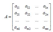
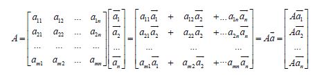
Where matrix A’s entry a11 refers to the matrix A’s row 1 column 1, a12 is A’s row 1 column 2, and keep going all the way to row 1 column n. Then matrix A goes down; entry a21 refers to row 2 column 1 of matrix A, and it continues down to row m column n. In fact, let us define some operations used by the matrix and vectors (x̅) to interact with each other. To do this, we take the product of the matrix and the calculated vector. The definition only works if A multiplied by the vector has the same number of components as A has columns. This is only valid for the vector that looks like this:
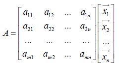
Where the vector (x̅) components are equal to the number of columns in the matrix A. Simply put, this product is A times the vector Ax̅ and is equal to
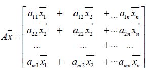
Where, the vector matrix corresponds to the first component of the matrix, times the first components of the vector, plus the second components of the matrix, times the second components of the vector, all the way to the nth component plus nth component.
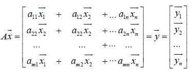
Here, we realize that the product is an A=m×n matrix, multiplying m by x̅ =n*1, and this is essentially the product of the vector of the column because the result is simply m*1. Now, based on this definition set, let us apply the matrix with the model’s actual components. For the group’s heading ā;
as well as for the coherence toward the center of the group b;
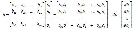
Where, the model’s primary elements gave the matrix A multiplied by the vector of group’s heading produces Aā, the matrix B is the coherence toward center of the b produces Bb. Inother words, if the main element of the model provided matrix A muliplied by the product of the group heading vector, then matrix B is consistent for the center of production B. The matrices A and B here are m×n (m rows and n columns) dimensional matrix of the same size, and each result is the simple product of the n×1 matrix of each n -dimensional vector, denoted by :
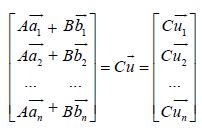
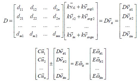
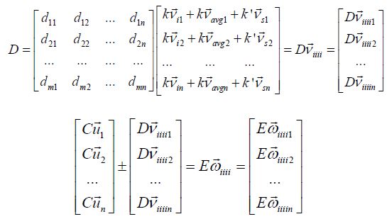
The matrices then include another quantity related to the individual’s current movement ū,
Here, multiplying the matrix D by the individual’s motion ν produces Dν, and the matrix Cūproduces Eω added by the Dν, or subtracted by Dν [when the new vector length of an individuals’ is less than that of a group].
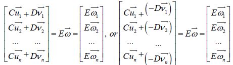
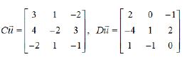
Here, the result Eω is simply m -dimensional vector, in that the number of n columns in each matrix has to match the dimension of each vector, and the new vector (Eω) matrix’s m rows has to be equal to the matrix rows in C and D. For example, with 3 x 3 matrices (3 basis inputs [columns] and 3 coordinates landing spots [rows]), if Cū and Dū,
show that 
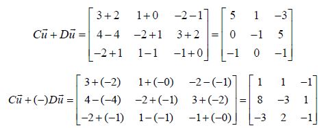
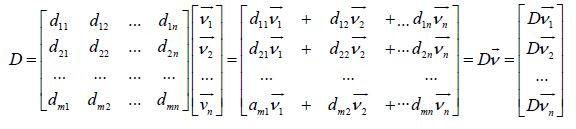
Using this product, the model assumes that the matrix-vector operations result in the subset of Dv with respect to the elements in ν decides the individual’s new position, while the āand b simply represent its averaged group quantities. Thus, as we explained in the mechanisms of the mathematical description, the operations of valid quantities depends on Rn (V ⊆ Rn) , so that the property of the subset becomes {Dν|ν∈V} , and the ν are as follows;
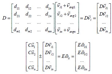
Here νi is the individual velocity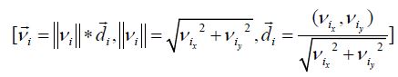 where the velocity of the individua
is represented by its size (‖vi‖ = the length of individual’s
magnitude) along with the direction of individual (di). The vavg is averaged velocity 1
where the velocity of the individua
is represented by its size (‖vi‖ = the length of individual’s
magnitude) along with the direction of individual (di). The vavg is averaged velocity 1
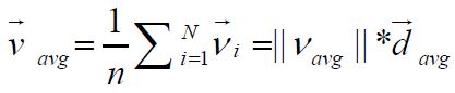 and covers the heading
of the entire population of individuals. All of the where Dv is equla to υi and υ
is a member of the V {νi | Dv =νi +ν ∈V} are valid. For
the product of the matrix by a scalar k [=IGT: the increase in the
individual’s velocity ( νi) resulted in a loss of group heading (vavg)]
[11], and the (1-|| k||)*νi+||k|| *vavg recorded is the matrix obtained
by multiplying each element by k.
and covers the heading
of the entire population of individuals. All of the where Dv is equla to υi and υ
is a member of the V {νi | Dv =νi +ν ∈V} are valid. For
the product of the matrix by a scalar k [=IGT: the increase in the
individual’s velocity ( νi) resulted in a loss of group heading (vavg)]
[11], and the (1-|| k||)*νi+||k|| *vavg recorded is the matrix obtained
by multiplying each element by k.
Observe that elements multiplied by k.
Next, for the network characteristics [12, 13], we denote vs=|| vs || *d s, where vs is a vector whose length ‖vs‖ and direction ds are a function of the Network Density (ND). Network density is calculated by measuring the actual connection (AC) and the Potential Connection (PC) of the network from its social ties [‖vs‖=ND=AC/PC, AC=(2*t)/N, PC=N(N-1)/2]. Here, the network density (‖vs‖) describes the potential connections of the network which are actual connections (AC/PC). The potential connection (PC=N(N-1)/2) is a connection that could potentially exist between two individuals irrespective of whether it actually does or not. This individual could know that individual; this object could connect to that one. Whether or not they do connect is irrelevant when we are talking about a potential connection. By contrast, an actual connection (AC=(2*t)/N) is one that actually exists. This individual does know that individual; this object is connected to that one. For example, in the living room of a house, connections could be 100% of all potential relationships. In contrast, the actual connections on a public bus are likely to be significantly lower than all the potential relationships because the number of people who actually know each other (actual connection) is probably low.
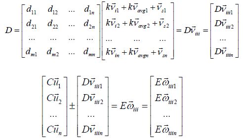
Here, the network characteristics are influenced by the mutation [14] rate (k’ = scalar) obtained by adding the corresponding
Reflect that even on a public bus, any individuals can connect
with any other, even if none of them know the other in their actual
connection (if one individual offers the highest payoff). In a house,
anyone can bring a guest into their living room. Here, the k’ controls
how fast the transition function propagates in the network, and how
fast the new position vector takes into account network density. That
could make the others modify the actual connection. The structural
instability of the dynamics of these small linear contributions can be interpreted as the network characteristics being influenced
by the exploration rate (k’ = scalar) which corresponds to a
mutation term in genetics. Finally, the model proposes to adopt
an existing possible interconnected relationship between the
network and its movement characteristics as another scalar 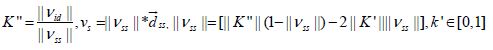 the product of the matrix B by a scalar k” obtained by
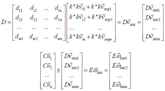
The fundamental properties of all combination are easily achieved via the operations of a matrix such as the one above. The model now considers an adoption probability which is given by an estimate of individuals’ velocity. Indeed, as no individual may know the exact value of a trait that has adopted the another individual’s velocity, this model yields that individuals can estimate the value at every schedule of each generation via a comparison p = [1+ eυ(πf −πr)]−1. Here πf is a velocity of the focal individual, πr is a velocity of a role individual, e denotes the exponential, and ω is an intensity of the selection. The focal individual imitates the velocity of the nearby role individual comparing its new position vector, and then the focal individual chooses to imitate the role individual’s strategy (ω < 1 = weak selection, ω→∞ = strong selection). The model applied this trait in three implementations (see Results section) each time expecting a different assessment of evolutionary patterns from the model mechanisms above.
Results
We can draw a number of conclusions regarding the operational principles mentioned in the mathematical description above. First, each individual’s velocity determines the change from timestep to timestep after its initial separation from any other individual. There is social learning about who needs to look for and copy its neighbors. The trade-offs are possible in the relationships between the number of individuals and the number of groups, and these are determined on the basis of a difficulty index that is a function of the ratio between the number of individuals and the number of groups. Their external properties come from network characteristics representing social ties, and mutations are related to how quickly the risk function propagates throughout the network. Indeed, the movement is affected by the trade-off between the direction of the individual velocity-group and and their actions, including theirnetwork properties, based on social ties multiplied by the rate of mutations. Such dynamics take into the relativity of the interactions of individual movements and their network characteristics as follows (Figure 1).

Figure 1: Estimation of the behaviour underlying internal (individual movement) characteristics: bias = scalar for IGT.
Note: The simulation shows that a displacement separates the individuals into a relative position structure controlled by the
average rate of exploration (See Figure 1 [left]). Although the pattern of the group behavior depends on a localized view of the
other individuals, it can be seen that a slight change in the individual movement characteristics based on the speed of heading
in their portraits significantly diverging (or converging). Group heading is lost due to increased individual velocity; Formula:
 represents the velocity of individuals. υavgis another vector quantity as the average velocity. μ is the result of an increase in the velocity of the individual (υi), resulting in a loss of group heading ( υavg), πr= role individual, πf = focal individual, and ω = selection intensity.
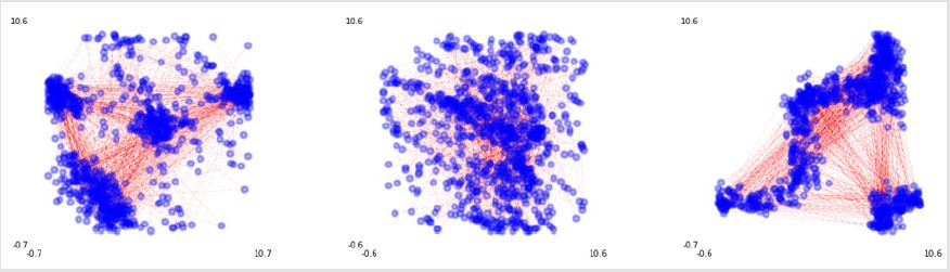
Figure 2.1: Estimation of the systemic risk based on external (mutation in network) characteristics, bias=scalar for mutation rate.
Note: To express this more quantitatively, the model attempts to apply network characteristics based on the mutation
rate (Reference to Figure 2.1 [left is the prototype with network characteristics, middle mutation 0.1, right 0.9]). Formula:  represents the velocity of individual. υavg is another vector quantity as
average velocity. μ is the trade-off as the individual’s velocity increases (υi) υs resulting in a loss of group heading ( υavg) is a vector with a network density, πr= role individual, πf = focal individual, and ω = selection intensity.
represents the velocity of individual. υavg is another vector quantity as
average velocity. μ is the trade-off as the individual’s velocity increases (υi) υs resulting in a loss of group heading ( υavg) is a vector with a network density, πr= role individual, πf = focal individual, and ω = selection intensity.
In the simulation, the plots show that a displacement separates the individuals into relative position controlled by the initial setting. Although the pattern of the group behavior depends on a localized view of the initial conditions, a slight change in individual kinetic characteristics based on individual-group trade-off means that the displacement significantly diverges (or converges); group heading is lost due to individual speed increase. (See Figure: blue dots represent their position in a x, y coordinate plane, and the red arrows denote their range with its density [the tone of color]). The Figure 2.1 show the social influence of network density multiplied by the mutation rate (left is the prototype with network characteristics, right shows high mutation). To put it more quantitatively, this diagram indicates that the behavior of modeled individual is more dynamic in social ties. (See Figure 2.2; the left plot shows patterns according to density (black and white) of social ties, while the right plot shows the distribution in three-dimensional space. Defaults = IGT =0.5, mutation = 0.5: left = social ties 0.4, middle = social ties 0.5, right = social ties 0.6).
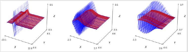
Figure 2.2: Fundamentals of external (social ties) characteristics: bias = scalar for social ties. Note: With the network density including social ties, the individual components seemed to indicate that the portrait is even more dynamic underlying the individual’s social ties (left = social ties 0.1, middle = social ties 0.5, right = social ties 0.9) in ℝ3 .
Finally, assessment of the strategy and evolution were measured based on their possible scenarios on how to mitigate behavioral problems. The prototype in the Figure 3 (plot of the left) shows an extreme case in the spectrum that applies a possible relation between difficult kinetic indexes divided by dynamic network characteristics. We observed the importance of interconnected interaction, as they are the main reason for re-unions of separate individuals. The group portraits appeared to change their pattern (See Figure 3 [middle-left and middle-right]) nonlinearly. Interestingly, the point at which the sudden changes occur is the point at which social ties both increase and the individuals become highly sensitive to small changes in the network’s social ties (Figure 3).
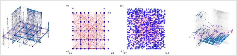
Figure 3: Possible scenario regarding behavior patterns. Meaningful results were achieved when the social relations were identical
to the mediating factor regarding the possible risk of the system. See Figure 3 right-hand side and left-hand side plots; in
R3 denotes average displacement of the individual’s position. Formula: 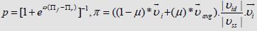 represents the velocity of an individual. υavg
is another vector quantity as the average velocity. μ is the trade-off as the individual’s
velocity increases (vi) resulting in a loss of group heading (vavg). |vid| is another scalar as a function of the ratio between
the two objects. |vss| is a length as a function of the network density, πr
= role individual, πf = focal individual, and ω = selection
intensity.
represents the velocity of an individual. υavg
is another vector quantity as the average velocity. μ is the trade-off as the individual’s
velocity increases (vi) resulting in a loss of group heading (vavg). |vid| is another scalar as a function of the ratio between
the two objects. |vss| is a length as a function of the network density, πr
= role individual, πf = focal individual, and ω = selection
intensity.
The simulation results show that changes occur at specific points as the social tie increase (See the middle right and left plots: blue dot = individuals, red line = links, background = density with symmetrical characteristics). Based on the defaults which the model set as an initial value (See Figure 3 left; St = 0.2, mutation = 0.5, IGT = 0.1, ID = 0.8), at the critical point (considered at st 0.55= middle left, 0.56 = middle right, 0.6= right, in this simulation), the system becomes highly sensitive to tiny changes in the network’s social tie. When relativity was applied, meaningful results were achieved, and the risk value of the social relations could be used as a mitigation factor against the possible heterogeneity of the system. With respect to heuristics through imitation-based social learning, the results suggest that individuals learn how to keep velocity d2 (α ) / dt2 = constant, α = acceleration] as a key factor for the homogeneity. Note that individuals are typically unaware that they are using this sort of heuristic, even though this accounts accurately for their behavior. Indeed, maintenance of a constant velocity between pursuer (focal model) and target (role model) has been found in a variety of animals besides humans, including bats, birds, fish, and insects. This was based on the available equivalent velocity (zero acceleration implied), but if the individual fails to keep to maintain the traits for the nearby individual, the displacement decays exponentially with uncertainty.
Discussion
This simulation shows how simple individual rules can lead to consistent group behavior, and how slight changes in those mechanisms can have a dramatic impact on an individual’s pattern (jeopardizing the whole system). It also shows how observations can be made beyond insufficient levels of complexity including learning and adaptation. This description deals with state per time as a determinant in neighbor allocation, and the number of neighbors placed at the location is based on the speed of movement (cultural evolution) scheduled for a given moment. As the agents represent individuals that occurred bottom-up, the actual state of their behavior tends to be more informative (agent-based modelling). This realistic simulation may allow the effects of different strategies of agents’ behavior to be tested and monitored (assessment of strategy and heuristic).
First, agent interactions are heterogeneous in this abstract setting. As the topology of the interaction movement trait can lead to significant deviations from the predicted pattern of behavior, it may generate various effects that mimic the behavior of real individuals in the social dynamics [15]. The individuals’ interactions are sensible decisions based on which the overall performance of the artificially designed system can be estimated and judged. The trade-off reliability between an individual and a group is primarily a measure of time variability of decision thresholds experienced by individual’s capability (see the implementation of Figure 1). In other words, we naturally differ in size, preference, and even strategy. The benefits of this model are clear; better and more efficient infrastructure planning, including compliance and better throughput due to the ability of the model to capture and reproduce emergent phenomena.
Second, there is a social network, that is, a structure and relationships between individuals that significantly impact their behavior. People transfer the control underlying their strategies to others; such irrational conformity often leads to cascading failures, such as dangerous overcrowding and slower escape or, more generally, physical damage (see the implementation in Figure 2). What might be called institutions are often subject to cognitive bias or systemic risks, and those biases has been blamed to a very large degree for unforeseen catastrophes and unexpected losses. In this simulation, collective behavior is an emergent phenomenon that occurs from relatively complex individual-level behavior and interactions between individuals. Collective behavior seems ideally suited to providing valuable insights into the mechanisms, and preconditions for, behavioral patterns according to their network characteristics (mutation rate and density of social ties). This model may suggest practical ways of mitigating the harmful consequences of such events and provide an optimal escape strategy. More directly, institutions need to be able to quantify their behavioral patterns within a reliable framework to be able to keep risk under control. Given the characteristics, this bottom-up simulation seems promising in terms of detecting cascading events and estimating the likelihood of potential losses (see implementation in Figure 3). An added benefit of simulation, then, is that one can identify where losses come from and test mitigation procedures: simulation can provide a thorough understanding of the capability (movement in the network) of the system drivers [4]. It also makes the formulation of mitigation strategies easier and can enable measurement of how the performance of the organization varies in response to these changes.
Third, let us suggest what might be evolvable heuristics for agents to assess their exposure to this systemic bias. Simple heuristics have an advantage in that they enable decisions to be made fast and with little information, and thereby avoid overfitting. The simulations may show that the structures of different interconnections affect which heuristics perform better, a relationship referred to as ecological rationality. This model proposes that the “gaze heuristic” can be a candidate that it works. According to researchers [16, 17], baseball players can use simple heuristics if a ball is already high in the air and travelling directly in line with the player. The player keeps his gaze on the ball, stars running, and adjusts his speed to ensure that the angle of the ball above the horizon appears constant [18]. The prediction is not that a player runs to a pre-computed landing spot and waits for the ball, but that the player is modified so that the image of the ball rises at a constant speed. It is possible that individuals do not compute velocity ( υ) at all even in this model but they have to reduce a maintained value of d2(υ) / dt2 in a systematic way. As υ increased, they would keep d2(υi) / dt2 at zero [ d2(υi) / dt2 = constant] [19]. Using this model, we might be able to propose such heuristics as evolvable traits or pay-off functions, guiding the evolution of these heuristics through imitation-based social learning. Note that individuals are typically unaware of using this sort of heuristic, even though this accurately accounts for their behavior. Such a rule of thumb from this simulation may provide us with more explicit examples of adaptation because individuals can be studied in the environments in which they evolved [20].
Fourth, to achieve homogeneity, the simulation adds diversity by incorporating simple relationships in the form of herd instinct which resembles natural individual behavior. To bring the mechanisms closer to the emergence, we applied explanatory structures with different bias that could be achieved with more complex heterogeneity. The bias in any system is a small, generally inconspicuous event that triggers a massive cascade in the network. On one level, the explanation for the risk is relatively simple and very unenlightening. However, these exist to trigger a more substantial response with a cascade that spreads fast, far, and wide without showing us much [13]. We investigate the systemic cascades by examining how the bias actually functions, creating mathematical logic which is extensively tested under evolutionary conditions (see mathematical description). One implication of this relatively simple model may go back to actual state evolution and the idea of a phase transition. Phase transitions are all very different from each other; for instance, the fact of ice melting to liquid water is embedded in that phenomenon as the idea of a critical point. The same goes for many sorts of things, such as dripping taps, animal populations, chemical reactions, and the behavior of markets.
The rules of thumb in this simulation may have suggested that an individual’s computational efficiency can be enhanced by operating near the critical point, which would mean that it is an adaptive feature [21]. We used well-accepted parameters connected to the system to try to determine if it was possible to describe the cascade by manipulating individual behavior and the key critical points. The mechanisms allow us to observe distinct types of behavior depending on how the parameters are connected and the threshold for when risk will fire in response to the applied rules and processes. As others have proved, this model may offer plausible insights into evolving patterns of network behavior, the strength of which is that it can bring some fresh perspective to understanding what the individual learns. This may be where the power of models comes into its own.
Conclusion
Users can design and run an infinite number of scenarios to observe the dynamics of the space, test the effectiveness of various management decisions, and track actor satisfaction over time. As the players in this model are customers (and attractions) with a behavior of their own, this can be a natural and very straightforward way of describing the system along the same lines. The use of various strategies, reinforcement learning, and other artificial intelligence techniques to generate strategies for agents can help gain fundamental insights into system dynamics [22]. The pattern of behavior emerges from the interactions of the actors, and individuals may alter in response to match in its their surrounding environment. Predicting how the pattern would change under a new set of operating regulations cannot be based on intuition or classical modelling techniques. Under these mechanisms, the system can be seen to exhibit a variety of hitherto unobserved dynamical behavior, including network characteristics and the coexistence of multiple search strategies.
Acknowledgements
This research was supported under the framework of International Cooperation Program managed by National Research Foundation of Korea (Grant Number: 2016K2A9A1A02952017).
References
- JA Marshall, PC Trimmer, Houston AI, Mc Namara (2013) On evolutionary explanations of cognitive biases. Trends in ecology & evolution 28(8): 469-473.
- Bonabeau E (2002) Agent-based modeling: Methods and techniques for simulating human systems. Proceedings of the National Academy of Sciences 99: 7280-7287.
- Daula T, Systemic Risk: Relevance, Risk Management Challenges and Open Questions.
- Leduc M, Poledna S, Thurner S (2017) Systemic risk management in financial networks with credit default swaps. available at SSRN 2713200.
- Helbing D (2013) Globally networked risks and how to respond. Nature 497(51): 7447.
- Trimmer PC, Houston AI, Marshall JA, Mendl MT, Paul ES (2011) Decision-making under uncertainty: biases and Bayesians. Animal cognition 14(4): 465-476.
- Sullivan O, Millington D, Perry J, Wainwright J (2012) Agent-based models–because they’re worth it? In Agent-based models of geographical systems.
- Helen C (2002) Modeling frameworks, paradigms, and approaches. Geographic Information Systems and Environmental Modeling, Prentice Hall, London, UK.
- Reynolds CW (1987) Flocks, herds and schools: A distributed behavioral model. In ACM SIGGRAPH computer graphics 21(4): 25-34.
- Oliva R (2016) Structural dominance analysis of large and stochastic models. System dynamics review 32: 26-51.
- Woodworth RS (1899) Accuracy of voluntary movement. The Psychological Review: Monograph Supplements 3: I.
- Demšar J, Lebar Bajec I (2013) Family bird: A heterogeneous simulated flock. Advances in Artificial Life, ECAL 12: 1114-1115.
- Traulsen A, Hauert C, De Silva Nowak, Sigmund K (2009) Exploration dynamics in evolutionary games. Proceedings of the National Academy of Sciences 106: 709-712.
- Santos FC, Pacheco JM, Lenaerts T (2006) Cooperation prevails when individuals adjust their social ties. PLoS computational biology pp. 1284-1291.
- Trimmer PC, Houston AI, Marshall JA, Mendl MT, Paul ES, et al. (2011) Decision-making under uncertainty: biases and Bayesians. Animal cognition 14: 465-476.
- McLeod P, Dienes Z (1996) Do fielders know where to go to catch the ball or only how to get there? Journal of experimental psychology: human perception and performance 22: 531-543.
- Oudejans R, Michaels CF, Bakker FC, Davids K (1999) Shedding some light on catching in the dark: Perceptual mechanisms for catching fly balls. Journal of Experimental Psychology: Human Perception and Performance 25: 531-542.
- Gigerenzer G (2004) Fast and frugal heuristics: The tools of bounded rationality. Blackwell handbook of judgment and decision making. Oxford, UK: Blackwell pp: 62-88.
- Dienes Z, Mc Leod P (1993) How to catch a cricket ball. Perception 22: 1427-1439.
- Johnson DD, Fowler JH (2011) The evolution of overconfidence. Nature 477: 317-320.
- Tversky A, Kahneman D (1986) Rational choice and the framing of decisions. Journal of business, 251-278.
- Iberall AS, Soodak H (1987) A physics for complex systems. In Self-organizing systems. Springer US pp. 499-520.
