The Spherical Inverted Pendulum with Pelvis Width in
Polar Coordinates for Humanoid Walking Design

Giuseppe Menga

info@biomedres.us +1 (720) 414-3554

One Westbrook Corporate Center, Suite 300, Westchester, IL 60154, USA

Biomedical Journal of Scientific & Technical Research

November, 2021, Volume 39, 5, pp 31641-31645

Review Article

The Spherical Inverted Pendulum with Pelvis Width in Polar Coordinates for Humanoid Walking Design

Giuseppe Menga*

Author Affiliations

Department of Control and Computer Engineering, Politecnico di Torino, Italy

Received: October 25, 2021 | Published: November 08, 2021

Corresponding author: Giuseppe Menga, Department of Control and Computer Engineering, Politecnico di Torino, Corso Duca degli Abruzzi 24, 10129 Torino, Italy

DOI: 10.26717/BJSTR.2021.39.006357

Abstract

The present communication is a follow up and extension of the paper “The Spherical Inverted Pendulum: Exact Solutions of Gait and Foot Placement Estimation Based on Symbolic Computation” by the same author. The walk design is approached by a 3-D inverted pendulum in a polar coordinate system. The advantage of this model is to easily offer indications of the energy expenditure of an efficient walk. However, the disadvantages that were never recognized by authors previously using this model is that the COG trajectory has to pass through the supporting foot location. This causes an unnecessary and unrealistic waving in the frontal plane during gait. The problem is discussed here and solved by extending the model of the inverted pendulum by introducing the pelvis width and the distance between the hips of the two legs, without adding dynamical complexity.

Keywords: Humanoid and Bipedal Locomotion; Legged Robots; Passive Walking; Foot Placement Estimation

Abbreviations: DOF: Degrees of Freedom; ZMP: Zero Moment Point; LIPM: Linearized Inverted Pendulum Model; SIP: Spherical Inverted Pendulum; FPE: Foot Placement Estimation

Introduction

Inverted pendulum models in 3-D have been used for balance and walk, since the beginning of the biped robotics era. Mostly, the two or three degrees of freedom (DOF) adopted for the pendulum were the two rotations around the horizontal axes and the length of the pendulum [1,2]. This configuration, by imposing the height of the COG to remain constant, allowed defining the linearized inverted pendulum model (LIPM). With this approximation the behaviors of the COG on the sagittal and frontal planes are independent and the celebrated zero moment point (ZMP) expression applies, linking linearly the ZMP position to the COG position and acceleration. Less frequently for the 3-D inverted pendulum the polar coordinate system was adopted, i.e. the rotation axes are the vertical and one of the horizontals. It has been noted that this configuration simplifies energy information, to be used for foot placement estimation (FPE) and walk design [3,4]. In a previous paper, this author used the 3-D inverted pendulum with polar coordinates, called spherical inverted pendulum (SIP), for generating an omnidirectional walk [5]. Comparing the resulting projection on the ground of COG trajectory and the supporting foot location using SIP with the classical biped walk based on controlling the ZMP, it was noted that in the sagittal plane, the two trajectories were similar, but in the frontal plane, they showed a marked difference. In fact, with the SIP model the COG trajectory passes always through the supporting foot position, creating an unnecessary large sway in the frontal plane during the gait.
This problem has been solved modifying the model, without additional dynamics. It has been introduced the pelvis width and the distance between the hips of the two legs. The approach is in the realm of passive walkers and of hybrid zero dynamics [6,7]. In particular, a similar model, with finite-width between the legs, was discussed previously in [8] and [9-11]. However, here the dynamics is simpler, and the progression of the walk is not obtained with a sloped ground, but with appropriate increments of the rotational velocities after the foot collision. Moreover, the inelastic collision is correctly approached as in the previous paper [5]. Finally, comparing with [9], global stability is controlled, in the style of FPE, simply by changing the angular speeds, the pelvis width and the angle α of the swing leg at the beginning of each step. The new model is presented in section 2, the transition from one-step to the next is discussed in section 3, some simulation examples are shown in section 4, and the last section 5 concludes the paper. In appendix, a generalization is introduced to be discussed in a future paper.

Modified Model of the SIP

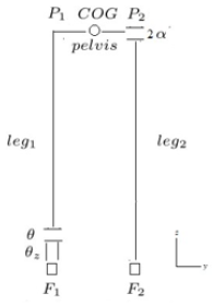
Figure 1: The modified spherical inverted pendulum.

The new model, with respect to the original SIP, adds in the pantograph the width of the pelvis and the distance between the hips of the two legs. Its kinematics is represented in (Figure1). The multibody is composed of three segments: the two legs and the pelvis. The two legs are massless. Only the pelvis, representing also the upper body, has a mass and an inertia. The supporting leg is fixed to the pelvis and offers the two degrees of freedom of the SIP represented by the joints of angles θ and θz. The swing leg is connected to the pelvis though the joint of angle 2· α. The angle 2· αz of the old model si not anymore needed, as the distance between the right and left feet is defined by the pelvis width. The characteristic points are the two feet (F1 and F2), the two hips (P1 and P2) and the COG. F1 is the supporting foot and F2 the swing foot. A parameter, called here “one”, assuming values ±1, accounts for right and left supporting foot in the hybrid simulation. As in the original SIP the motion angles are θ, θz. 2 · α defines the angle of the swing foot and is constant during a step. The dynamical model is of order 10 with configuration variables θz, θ, x, y, z, where x, y, z are the coordinates of the pivot foot, and corresponding motion variables γ, ω, u1, u2, u3. However, a non-holonomic constraint imposes a fixed position of the pivot foot: u1 = u2 = u3 = 0 during the swing, and it is released at the collision of the swing foot with the ground to determine γ+, ω+, u1 +, u2 +, u3 +. For all the details of the dynamics, refer to the father paper [5].

Switching Supporting Foot and Ground Collision

For future extensions, the switching of feet has been computed, in the most general way, by equating, through non-linear least squares, the direction cosines matrix of the swing leg frame at the touch down in terms of orientation angles in the body coordinate frame 3-2-1 (ZYX), and assigning the first two coordinates to θz and θ of the new supporting leg. See the appendix A. The touch down is given when the vertical position of foot F2 reaches the ground, and the inelastic collision defines γ+ and ω+, as in the previous paper.

Simulation Examples

In this section, a few simulation examples are shown (Figures 2-4) assigning the same initial conditions and different pelvis widths and strategies adopted for regenerating the γ rotational speed after collision at the start of a new step. In particular, γ, along with the pelvis width, controls the distance between feet and the sway of the COG in the frontal direction, α and ω0, mostly, control step length and cadence, respectively. Figure 2 shows the limitations of the original SIP, irrespective of the speed regeneration strategy adopted. The tracking of an omnidirectional trajectory of (Figure 5) is obtained controlling γ at the beginning of each step to follow the desired path. With strategy a), at each step after the switching γ maintains the same natural value given after the collision (γ = γ+). With strategy b), irrespective of the value obtained after the collision, γ is set to the constant initial value (γ = γ0).

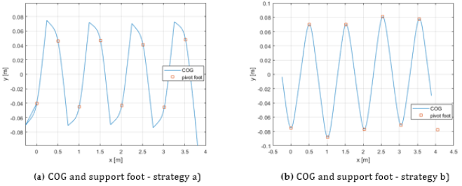
Figure 2: Behavior of COG with pelvis width equal 0 m.

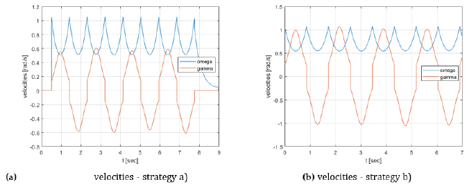
Figure 3: Behavior of angular velocities with pelvis width equal 0 m.

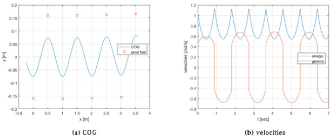
Figure 4: Behaviors with pelvis width equal 0.17 m, and regeneration strategy b).

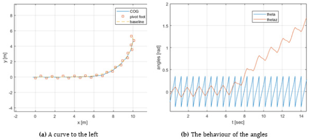
Figure 5: Omnidirectional gait.

Conclusion and Future Work

The classical pendulum in polar coordinates limits the COG trajectory to pass through the pivot foot position. This is unrealistic. The problem is solved by introducing the width of the pelvis, and the distance between the hips of the two legs. However, in the most general case the DOF of the pendulum have to be increased to take into account the rotation along the x-axis of the pelvis, non-existing in the original SIP model. A special case, when the swing foot is not rotated along its z-axis, which doesn’t introduce rotation of the pelvis along its x axis and maintains the dynamical complexity identical to the classical model, is considered in this paper. The general framework si introduced in the appendix, and it will be considered in a future paper.

Appendix A - Switching Pivot Feet - a General Framework

The simplicity of the approach presented in this paper relies on the fact that the frame of leg2 has not rotation along his z axis; for this and the assumption of flat ground the pelvis has no rotation along the x axis and its revolution along the y axis can be resettled at each step. Situation changes if, as example, the angle αz is added to the swing leg, as in the original SIP model, or the ground is not flat. To maintain the consistency of the COG position and the pelvis orientation at the switching, the dynamics of the pendulum increases to 3 DOF with motion angles θz, θ and θx , and two joints are added to the kinematics, with fixed angles at each step, α1 and αz1 (Appendix A1). Then at the switching, α1 = α, αz1 = αz, and the initial values of θz, θ and θx are obtained equating the direction cosine matrix of leg2 to a frame with direction angles defined in the body coordinate frame 3-2-1 (ZYX). Indicating with N_Leg2 the direction cosines matrix from the inertial N to the Leg2 frames, it can be written as:

N_Leg2(1, 1) = cos()·cos(z)
N_Leg2(1, 2) = sin(z)·cos()
N_Leg2(1, 3) = -sin()
N_Leg2(2, 1) = sin(x)·sin()·cos(z) - sin(z)·cos(x)
N_Leg2(2, 2) = cos(x)·cos(z) + sin(x)·sin()·sin(z)
N_Leg2(2, 3) = sin(x)·cos()
N_Leg2(3, 1) = sin(x)·sin(z) + sin()·cos(x)·cos(z)
N_Leg2(3, 2) = sin()·sin(z)·cos(x) - sin(x)·cos(z)
N_Leg2(3, 3) = cos(x)·cos()

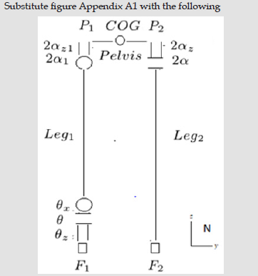
Appendix A1: The spherical inverted pendulum with pelvis width - a general framework.

References

- S Kajita, F Kanehiro, K Kaneko, K Yokoi, H Hirukawa (2001) The 3D Linear Inverted Pendulum Mode: A simple modeling for a biped walking pattern generation. 2001 IEEE/RSJ International Conference on Intelligent Robots and Systems Maui, Hawaii.
- S Kajita, F Kanehiro, K Kaneko, K Fujiwara, K Harada, et al. (2003) Biped Walking Pattern Generation by using Preview Control of Zero-Moment Point. 2003 IEEE International Conference on Robotics & Automation Taipei, Taiwan, September, p. 14-19.
- BJ DeHart (2019) Dynamic Balance and Gait Metrics for Robotic Bipeds. doctoral thesis University of Waterloo.
- BJ DeHart, R Gorbet, D Kulic (2018) Spherical Foot Placement Estimator for Humanoid Balance Control and Recovery. 2018 IEEE International Conference on Robotics and Automation (ICRA).
- G Menga (2021) The Spherical Inverted Pendulum: Exact Solutions of Gait and Foot Placement Estimation Based on Symbolic Computation. Appl Sci 11(4): 1588.
- S Collins, A Ruina, R Tedrake, M Wisse (2005) Efficient bipedal robots based on passive-dynamic walkers. Science 307: 1082-1085.
- Arthur de Oliveira, Guilherme Vicinansa, Paulo da Silva, Bruno Ang’elico (2019) Frontal Plane Bipedal Zero Dynamics Control. arXiv: 1904. 12939.
- K Miyahara, Y Harada, DN Nenchev, D Sato (2019) Three–Dimensional Limit Cycle Walking with Joint Actuation. The 2009 IEEE/RSJ International Conference on Intelligent Robots and Systems October, p. 11-15.
- A Jaberi, MR Hairi Yazdi, MR Sabaapour (2015) Analysis of 3D Passive Walking Including Turning Motions for the Finite-width Rimless Wheel. JAMECH 46(1): 63- 68.
- AD Ames, EA Cousineau, MJ Powell (2012) Dynamically stable bipedal robotic walking with NAO via human-inspired hybrid zero dynamics. HSCC ’12: Proceedings of the 15th ACM international conference on Hybrid Systems: Computation and Control, pp. 135-144.
- A Hereid, EA Cousineau, CM Hubicki, AD Ames (2016) 3D dynamic walking with underactuated humanoid robots: A direct collocation framework for optimizing hybrid zero dynamics. 2016 IEEE International Conference on Robotics and Automation (ICRA).