Chemical Spots and Vortices Caused By the Current-Driven Diffusion in Plasma Volume 2 - Issue 2

Vadim Urpin*

• AF Ioffe Institute of Physics and Technology, Russia

Received: January 25, 2018;   Published: February 08, 2018

Corresponding author: Vadim Urpin, AF Ioffe Institute of Physics and Technology, Russia

DOI: 10.26717/BJSTR.2018.02.000744

Abstract PDF

We consider diffusion caused by a combined influence of the electric current and Hall effect, and argue that such diffusion can form in homogeneities of a chemical composition in plasma. Such current-driven diffusion can be accompanied by prop-agation of a particular type of waves in which the impurity number density oscillates alone. These compositional waves exist if the magnetic pressure in plasma is greater than the gas pressure.

Keywords: Plasma magnetic fields; Plasma waves; Plasma chemical spots

Often laboratory and astrophysical plasmas are multicomponent, and diffusion plays an important role in many phenomena in such plasmas. For instance, diffusion can be responsible for the formation of chemical inhomogeneities which influence emission, heat transport, conductivity, etc see, e.g., [1-3]. In fusion experiments, the source of trace elements is usually the chamber walls, and diffusion determines the penetration depth of these elements and their distribution in plasma see, e.g., [4-6]. Even a small admixture of heavy ions increases drastically radiative losses of plasma and changes its thermal properties. In astrophysical conditions, diffusion leads to the formation of element spots detected on the surface of many stars see, e.g., [7-9].

Diffusion in chatged gases or fluids can differ qualitatively from that in media con-sisting of neutral paticles because of the presence of electrons and electric currents. A mean motion of electrons caused by electric currents provides an additional internal force those results in diffusion of trace elements. One more important contribution of electrons in diffusion is relevant to the Hall effect. The magnetic field can magnetize the charged particles that lead to anisotropic transport. In the case of electron transport, such anisotropy is characterized by the Hall parameter, x_e = ω_Beτ_e where ω_Be = eB /m_ec is the gyrofrequency of electrons and τ_e is their relaxation time; B is the magnetic field. In a hydrogen plasma, τ_e = 3^√m_e (k_bT )^3/2 / 4^√2πe⁴n∧ see [10] where n and T are the number density of electrons and their temperature, respectively, A is the Coulomb logarithm. At x_e ≥ 1, the rates of diffusion along and across the magnetic field become different and, in general, diffusion can lead to the inhomogeneous distribution of elements.

In this paper, we consider the diffusion process that can lead to formation of chemical inhomogeneities in plasma. This process is caused by a combined influence of electric currents and the Hall effect. Using a simple model, we show that the interaction of the electric current with trace elements leads to their diffusion in the direction perpendicular to both the electric current and magnetic field. This type of diffusion can alter the distribution of chemical elements in plasma and contribute to formation of chemical spots even if the magnetic field is relatively weak and does not magnetize electrons (x_e «: 1). We also argue that the current-driven diffusion in combination with the Hall effect can be the reason of the particular type of modes in which the number density of a trace element oscillates alone. The considered diffusive process is rather general and can be important in any medium consisting of charges particles.

Consider plasma with the magnetic field parallel to the axis z, B = ^B ~ e_z, where (s, ϕ, z) are cylindrical coordinates and ( ~ e_s,~ e_ϕ,~ e_z) the corresponding unit vectors, respectively. We assume that plasma is cylindrical and the magnetic field depends on the cylindrical radius alone, B = B (s) . Then, the electric current is given by

We suppose that j_ϕ → 0 at large s and, hence, B → B₀ = const at s → ∞ . Note that the dependence B(s) cannot be an arbitrary function of s because, generally, the cylindrical magnetic configurations are unstable if B(s) increases with s or decreases sufficiently slowly see, e.g., [11-13]. In real conditions, the magnetic field has a more complex topology than our simple model. However, our model describes correctly the main qualitative features of current-driven diffusion and, in some cases; it can even mimic real magnetic fields see, e.g., [14]. We assume that plasma consists of electrons e, protons p, and a small admixture of heavy ions i. The number density of species i am small and it does not influence dynamics of plasma. The partial momentum equations in fully ionized multicom-ponent plasma have been considered by a number of authors see, e.g., [15]. The momentum equation for particles α (α = e, p, i) reads

The dot denotes the partial time derivative. Here, m_α and Z_α are the mass and charge number of particles α, n_α and p_α are their number density and pressure, respectively, V_α is the mean velocity, F_α is an external force acting on the particles α; E and B are the electric and magnetic fields, respectively: R_α is the internal friction force caused by collisions of particles a with other sorts of particles. Since R_α is the internal force, the sum of R_α over a is zero in accordance with Newton’s third law. We neglect the influence of F_α because it is usually small.

If there are no mean hydrodynamic velocity and only diffusive velocities of trace elements are non-vanishing, the partial momentum equation for particles α reads

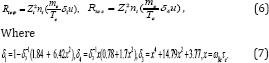
The friction forces R_i for trace particles i can be represented as R_i = R_ie + R_ip where the force R_ie is caused by scattering of ions i on electrons and R_ip by scattering on protons. If n_i « n_p , R_ie is given approximately by

Where is the force acting on the electron gas [15]. In this case, is determined by Scattering of electrons on protons but scattering on ions i gives a small contribution. Therefore we can use for the expression for [15] for hydrogen plasma. In our model, this expression reads

Where is the deference between the mean velocities of electrons and protons α_⊥ , α_∧ , β_⊥^uT and β_⊥^uT are coefficients calucated by [15-18] b = B/B. The first two terms on the r.h.s. of Eq. (11) describe the standard friction force caused by a relative motion of the electron and proton gases. The last two terms on the r.h.s. of Eq. (11) represent the so-called thermoforce and are vanishing if ∇T = 0. Taking into account that ~ u = u ~ e_ϕ in our model and using Coefficients α_⊥ and α_⊥ calculated by [15], we obtain the following expressions for the cylindrical components of R_ie

The force consists of two parts as well, and which are proportional to the relative velocity of ions i and protons and to the temperature gradient, respectively. The thermoforce is vanishing in our model. The Friction force is given by

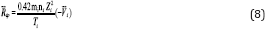
See [16] Where, 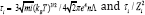is the characteristic timescale of ion-proton scattering; we assume that Coulomb logarithms are the same for all types of scattering. The momentum equation for the species i (see Eq. (3)) contains components of the electric field, E_s and E_ϕ. These components can be determined from the momentum equations (3) for electrons and protons. Taking into account the condition of hydrostatic equilibrium and quasi-neutrality (n_e ≈ n_p), we obtain the following expressions for the radial and azimuthal electric fields.

Substituting Eqs.(6), (8), and (9) into Eq.(3) for the trace particles i, we arrive to the expression for a diffusion velocity V_i,

V_nI Are the velocities of ordinary diffusion and V_B and Viϕ are the radial and azimuthal diffusion velocities caused by the electric current. The corresponding diffusion coefficients are

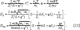
Eqs. (10)-(12) describe the drift of ions i under a combined influence of ∇n_i and . If magnetic field is weak and x « 1, then Eq.(12) yields ⁱ

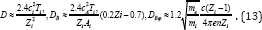
Where c²_A = B²1(4πnm_p) [16], The Coefficients D is always positive but two other diffusion Coefficients can be positive or negative depending on the parameters of plasma. In the opposite case of a very strong magnetic field, q ≫ 1, Eq.(12) yields.

In a strong field, diffusion in the radial direction is suppressed because all sorts of particles are magnetized. For instance, the Coefficients D (Eq. (14)) and the corresponding diffusion velocity V_ni which characterize the standard diffusion in the s-direction are ≈ q² » 1 times smaller than those in the case of a weak magnetic field. The Coefficients DB is also approximately q² times smaller in a strong magnetic field. Note that D_B reaches saturation and do not depend on the field strength at q»1. If the electric current is fixed (dB/ds =const), the radial diffusion velocity V_B caused by currents decreases ∞ 1/ B. As far as the azimuthal diffusion is concerned, the Coefficients D_Bϕ does not depend on the magnetic field in both cases, strong and weak magnetic fields. However, D_Bϕ in a strong field is greater by a factor .

It is generally believed that standard diffusion smoothes chemical inhomogeneities on a diffusion timescale ~ L² / D where L is the length scale of a non-uniformity. This is not the case, however, for diffusion given by Eq. (12). In this case, chemical inhomogeneities can exist during a much longer time than ~ L² /D because the equilibrium distribution is reached due to balance of two diffusion processes, standard (∞∇n_i) and current-driven ( ∞dB / ds) ones, which push ions in the opposite directions. As a result, V_is = 0 in the equilibrium state and this state can be maintained as long as the electric current exists. Note that the radial velocity is vanishing in the equilibrium state but the azimuthal velocity is non-zero in this state. It turns out that impurities rotate around the magnetic exist even if equilibrium is reached. The direction of rotation depends on the sign of dB/ds and is opposite to the electric current. Since electrons move in the same direction, heavy ions turn out to be carried along the flow of electrons. Different ions move with different velocities around the axis. If the magnetic field is weak (x ≪ 1), the difference between different sorts of ions ∇V_iϕ is of the order of

Where B₄ = B/10⁴G , n₁₄ = n/10¹⁴ cm^-3, and L₁₀ = L/10¹⁰cm . Since different impurities rotate around the magbetic axis with different velocities, periods of such rotation also are different for different ions. The difference in periods can be estimated as

If the distribution of impurities is non-axisymmetric then such diffusion in the azimuthal direction should lead to slow variations in the abundance peculiarities. Note that in the case of a strong field (q »1) all sorts of trace particles rotate around the axis with the same period that depends only on the number density and electric current. The condition of hydrostatic equilibrium in our model is given by

Where p and ρ are the pressure and density, respectively. Since the background plasma is hydrogen, p ≈ 2nk_BT where k_B is the Boltzmann constant? Integrating the s-component of Eq. (13) and taking into account that the temperature is constant in our model, we obtain

Where β= 8π_o/B²; (p₀, n₀, T₀, β₀) are the values of (p,n,T,β) at S → ∞. Consider the equilibrium distribution of trace elements in cylindrical plasma. In equilibrium distribution, we have V_is =0 and Eq.(10) yields

The term on the r.h.s. describes the effect of electric currents on the distribution of trace elements. We consider first the case of a weak magnetic field with x ≪ 1. Then, one has from Eq. (17)

Substituting Eq. (19) into Eq.(18) and integrating, we obtain

And n_i0 is the value of n_i at s → ∞. Denoting the local abundance of the element i as γ_i = n_i/ n and taking into account Eq. (17), we have

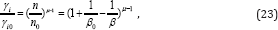
Where, γ _i0 = n_i0 /n₀ Local abundances turn out to be flexible to the field strength and, particularly, these concerns the ions with large charge numbers. If other mechanisms of diffusion are negligible and the distribution of elements is basically current- driven, then the exponent (μ-1) can reach large negative values for elements with large Z_i and, hence, produce strong abundance anormalies. For instance, (μ -1) is equal 1.16, -0.52, and -2.04 for Z _i =2, 3, and 4, respectively. Note that (μ - 1) changes its sign as z _i increases: (μ-1) > 0 if z_i = 2 but (μ-1) < 0 for Z_i ≥ 3. Therefore, elements with Z_i ≥ 3 are in deficit (γ < γ_i0) in the region with a weak magnetic field (B < B₀) but, on the contrary, these elements should be overabundant in the region where the magnetic field is stronger than B₀.

A distribution of the impurities can be substantially different if the magnetic field is strong and q ≫ 1. Using the same procedure as in the case of a weak field, we obtain

Therefore, all trace elements with Zi > 1 are overabundant in the regions with the magnetic field weaker than B0. On the contrary, these elements are under abundant in the regions with a stronger magnetic field.

In our simplified model of plasma cylinder with the velocity given by Eq.(10), the continuity equation for trace ions i reads

Consider the behaviour of small disturbances of the number density of trace ions by making use of a linear analysis of Eq. (25). In the basic (unperturbed) state, plasma is assumed to be in diffusive equilibrium and, hence, the unperturbed impurity number density satisfies Eq. (19). Since the number density of impurity i is small, its influence on parameters of the basic state is negligible. For the sake of simplicity, we consider disturbances that do not depend on z. Denoting disturbances of the impurity number density by δn_i and linearizing Eq.(25), we obtain the equation governing the evolution of such small disturbances,

For the purpose of illustration, we consider only disturbances with wavelengths shorter than the length scale of unperturbed quantities. In this case, we can use the so called local approximation for a consideration of linear waves and assume that small disturbances are ∞ exp (-iks - iMϕ) where k is the wave vector (ks» 1) and M is the azimuthal wave number. Since the basic state does not depend on time, δn_i can be represented as δn_i ∞ e^{iωt-iks-iMϕ} where ω should be calculated from the dispersion equation. Substituting δn_i in such form into Eq. (26), we obtain the following dispersion equation

This dispersion equation describes spiral waves in which only the number density of impurities oscillates and, therefore, such waves can be called "compositional". The quantity ω_R characterizes decay of these waves with the characteristic timescale ~ (Dk² )^-1 typical for a standard diffusion. The frequency ω_I describes oscillations of impurities caused by the combined action of electric current and the Hall effect. Note that ω_I can be of any sign but ω_R is always positive, the frequency ω_S characterizes oscillations in the radial direction and ω_ϕ in the azimuthal direction. The compositional waves are a periodic if ω_R > |ω_I| and oscillatory if |ω_i| > ω_R. We consider the compositional waves in particular cases of weak (x « 1) and strong (q»1) magnetic fields. Weak magnetic field (x « 1), If ks » M (radial waves), the condition | ωI |> ωR in a weak field is equivalent to

Where and c_s is the sound speed, c ²_s = k_BT / m_p .In the opposite case M » ks (azimuthal waves), the compositional waves are oscillatory if

Both conditions (28) and (29) require the magnetic field such strong that the magnetic pressure is substantially greater than the gas pressure. The frequency of com-positional waves is higher in the region where the magnetic field has a stronger gradient or, in other words, where the density of electric currents is greater. Note that different impurities oscillate with different frequences. Consider first the radial waves with M = 0. Substituting M = o into Eq. (27), we obtain the dispersion equation for such waves in the form

This dispersion equation describes waves in which only the number density of trace particles oscillates and oscillations of n_i occur only in the radial direction. The order of magnitude estimate of ω_S yields

Where l _i = c_iτ_i i s the mean free-path of ions i. Note that different impurities oscillate with different frequences. Therefore, if there are several sorts of trace ions in plasma, the chemical structure should exhibit variations of local abundances under the influence of compositional waves. The dispersion equation for non- axisymmetric waves with M ≫ ks reads in a weak field

In non-axisymmetric waves, trace ions rotate around the cylindrical axis with the frequency ω_ϕ and decay slowly on the diffusion timescale ~ ω_R^-1 . The frequency of such waves is typically higher than that of radial waves. One can estimate the ratio of these frequencies as

Since these estimates are justified only in the case of a weak magnetic field (x ≪ 1), the period of non-axisymmetric waves is shorter for waves with M > A_ix(ks). The ratio of diffusion timescale and period of non-axisymmetric waves is

And can be large. Therefore, azimuthal waves can be oscillatory as well.

Strong magnetic field (q »1) in a strong magnetic field, the order of magnitude estimates of the characteristic frequences are

Like the case of a weak field, the frequency of compositional waves is higher in the region where the density of electric currents is greater. Oscillations of different trace ions occur with different frequences in radial waves but azinuthal oscillations have the same frequency for different impurities. The frequency of azimuthal waves is higher than that of radial waves if

If the magnetic field is such strong that q >> 1 then the azimuthal waves oscillate with a higher frequency than the radial ones even for not very large M. The condition that radial waves exist in a strong magnetic field, |ω_S| ≫ ω_R |, is given by

Like the case of a weak magnetic field, compositional waves occur in plasma only if the magnetic pressure is greater than the gas one. The analgous condition for azinuthal waves, ω _ϕ » ω_R , reads

Note that this condition can be satisfied even if the magnetic pressure is smaller than the gas one but q and M are large.

We have considered diffusion of heavy ions under the influence of electric currents. Generally, the diffusion velocity in this case can be comparable to or even greater than that caused by other diffusion mechanisms. The current-driven diffusion can form chemical inhomogeneities even if the magnetic field is relatively weak whereas other diffusion mechanisms require a substantially stronger magnetic field. The current-driven diffusion is relevant to the Hall effect and, therefore, it leads to a drift of ions in the direction perpendicular to both the magnetic field and electric current. As a result, a distribution of chemical elements in plasma depends essentially on the geometry of the magnetic fields and electric current. Chemical inhomogeneities can manifest themselves, for example, by emission in spectral lines and a nonuniform plasma temperature. Usually, diffusion processes play an important role in plasma if hydrodynamic motions are very slow. In some cases, however, chemical spots can be formed even in flows with a relatively large velocity but with some particular topology (for example, a rotating flow).

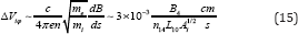
Our study reveals that a particular type of waves may exist in multicomponent plasma in the presence of electric currents. These waves are slowly decaying and characterized by oscillations of the impurity number density alone. They exist only if the magnetic field is such strong that the magnetic pressure is greater than the gas pressure. Generally, the frequency of such waves turns out to be different for different impurities. This frequency is rather low and is determined mainly by a diffusion timescale. If M = 0, it can be estimated as where λ = 2π/ k is the wavelength of waves. In astrophysical conditions, such waves can manifest themselves in the atmospheres of magnetic stars where the magnetic field is of the order of 10⁴ G and the number density and temperature are 10¹⁴ cm^-3 and 10⁴ K, respectively. If the length scale, L, and the wavelength, λ, are of the same order of magnitude (for in-stance, cm), then the period of compositional waves is yrs. This is much shorter than the stellar lifetime (see, e.g., [17, 18]) and generation of such waves in the atmospheres should lead to spectral variability with the corresponding timescale.

Compositional waves can occur in laboratory plasmas as well but their frequency is essentially higher. If B~ 10⁵G, n~ 10¹⁵cm ³ , T~ 10⁶K , and L~λ~10² cm, then the period of compositional waves is ~ 10^-8 s . Note that this is only the order of magnitude estimate but frequencies of various impurities can differ essentially since the period of compositional waves depend on the sort of heavy ions. In terrestrial conditions, the compositional waves also can manifest themselves by oscillations in spectra. Note that these waves exist only if the magnetic pressure is greater than the gas pressure. The current-driven diffusion can be important not only in plasma but in some conductive fluids if the magnetic field is sufficiently strong there.

1. Vekshtein G (1987) In Review of Plasma Physics. B Kadomtzev (Eds.). Consultants Bureau, NY,USA, 15: 1.
2. Ren Y, Yamada M, Ji H, Gerhardt S, Kulsrud (2008) Phys Rev L 101: 5003.
3. Kagan G, Tang XZ (2012) Comment on Plasma adiabatic lapse rate. Ph Rev Lett 107: 50030.
4. Losseva T, Popel S, Yu MY, Ma J X (2007) Ambipolar diffusion in complex plasma. Phys Rev E75(2): 046403.
5. 5. Ott T, Bonitz M (2011) Diffusion in a strongly coupled magnetized plasma. Phys Rev L 107(13): 135003.
6. Molvig K, Vold E, Dodd E, Wilks S (2014) Nonlinear structure of the diffusing gas-metal interface in a thermonuclear plasma. Phys Rev L 113(14): 145001.
7. Khokhlova V (1985) Sov Sci Rev (Sec E: Astrophysics and Space Phys Reviews) 4: 99-159.
8. Mathys G, Hubrig S (1995) Magnetic fields of the HgMn spectroscopic binaries X LUPI and 74 Aquarii. A&A 299: 810-814.
9. Kochukhov O (2004) IAU Symposium 224,433.
10. Spitzer L (1978) Physical Processes in the Interstellar Medium Wiley, New York, USA.
11. Tayler RJ (1973) the adiabatic stability of stars containing magnetic fields-I Toroidal fields. MNRAS, 161: 365.
12. Bonanno A, Urpin V (2008) Non-axisymmetric instability of axisymmetric magnetic fields. A&A 488(1): 1-7.
13. Bonanno A, Urpin V (2011) the magneto hydrodynamic instability of current-carrying jets. Phys Rev E84: 6310.
14. Urpin V, Chanmugam G, Sang Y (1994) the magneto rotational and Tayler instabilities in the pulsar magnetosphere. ApJ 433: 780.
15. Braginskii S (1965) In Reviews of Plasma Physics. In: M Leontovich (Eds.). Consultants Bureau, New York, USA, P. 1,205.
16. Urpin V (2015) Element spots in Ap and Hg-Mn stars from current- driven diffusion. Astron Nachr 336(3): 266-270.
17. Bhattacharya D, Van den Heuvel EPJ (1991) Formation and evolution of binary and millisecond radio pulsars. Phys Rep 203(1-2): 1-124.
18. Urpin V, Konenkov D, Geppert U (1998) Evolution of neutron stars in high-mass X-ray binaries. MNRAS 299(1): 73-77.