Site-Specific Leaching Map of a Salt Affected Soil in Egypt Volume 2 - Issue 4

Sameh M Shaddad*¹ and Mohamed Y Hendawi²

• ¹Soil science department, Zagazig University, Egypt
• ²Plant protection department, Zagazig University, Egypt

Received: February 15, 2018;   Published: February 22, 2018

*Corresponding author: Sameh M Shaddad, Soil science department, Zagazig University, Egypt

DOI: 10.26717/BJSTR.2018.02.000791

Abstract PDF

Geostatistical techniques allow detecting soil spatial variability and applying site-specific management in a way that traditional methods do not. The study objective was to develop a prescription map for leaching requirements (LR) of a field in Sharkia governorate in Egypt using ordinary kriging as interpolator. 91 soil samples were collected and subjected to electrical conductivity analysis (ECe). All data were randomly divided into two subsets named as calibration and validation. Prediction performance was assessed by calculating two statistics: mean error (ME) and mean standardized squared error (MSSE). Results showed that the ME and MSSE values were 0.09 and 1.27 in validation. LR was calculated for zones having ECe greater than 4 dS.m^-1 to reach 2 dS.m^-1 and was 3625 and 1149 m3. Results showed that assuming the ECe mean value for 91 soil samples (5.12 dS.m^-1) - without geostatistical interpolation - a quantity of 6203 m3 of water should be added to reduce salinity of the whole field to 2 dS.m^-1. So 1429 m3 can be saved and then used for irrigation. These results emphasize the importance of geostatistics in detecting within field variability and hence applying site-specific management especially in countries suffering from water scarcity.

Keywords: Soil salinity; Site-specific management; Ordinary kriging

Abbrevations: LR: Leaching Requirements; ECA: Electrical Conductivity Analysis; ME: Mean Error; MSSE: Mean Standardized Squared Error; BLUE: Best Linear Unbiased Estimator

Soil salinity is a crucial problem facing countries in arid and semi arid regions which negatively affects sustainable agriculture Eilers et al. [1]. This problem needs to be accurately quantified and mapped in order to mitigate and control its negative effects Herrero and Perez-Coveta [2]; Benyamini et al. [3]; Wang [4] especially in irrigated soils Amezketa [5]. Soil salinity cab be solved by leaching soluble salts from the root zone by adding water with good drainage conditions. In Egypt, salt-affected soils are located in the Northern- Central part of the Nile Delta and on its Eastern and Western sides. Also, in Wadi El-Natroun, El-Kebeir, the Oases, many parts of the Nile Delta and Valley and El-Fayoum province are characterized as salt affected soils. In Egyptian irrigated lands, about nine hundred thousand hectares suffer from salinization. These are distributed as follows: 60 % is in Northern Delta, 20 % in Southern Delta and Middle Egypt and 25 % in Upper Egypt FAO [6]. Conventionally, data of soil properties are summarized by averages of collected soil samples with no consideration of the spatial variation either at macro scale or at micro scale (within-field) (Webster and Oliver [7] and Navarro-Pedreno et al. [8].

Geostatistics provides good tools in capturing within field spatial variation of soil variables that is used to delineate management zones and consequently know where and how much farm inputs should be added Oliver and Webster [7]. Geostatistical methods are non-destructive, time saving and cost effective as comparing with traditional methods and provide fine- scale information about soil variables. Spatial distribution of soil properties has been recognized by various researchers Burgess and Webster [9]; Warrick et al. [10]; Odeh et al. [11]; Juang & Lee [12]. Oridinary kriging as a geostatistical interpolation method was the most common used to predict and map soil parameters at unsampled locations Lopez-Granados et al. [13]; Meul & Van Meirvenne [14]; Sumfleth & Duttmann [15]. This study aimed at assessing the spatial distribution and predicting soil salinity over a field in Sharkia governorate using ordinary kriging for the purpose of preparing a prescription map of leaching requirements.

Site Description, Sampling and Laboratory Analysis

This study was conducted in 4.6 ha field (30° 51' 53.31” N, 32° 02' 50.45” E), located in Bahrelbaqar, Sharkia governorate. A total of 100 soil samples based on an almost regular 25x25 m grid at 0. 20 m depth were collected and transported to the soil laboratory, where they were dried, ground and sieved with a 2 mm sieve and electrical conductivity (EC) was measured. EC was measured in 1:5 soil water extract according to Jackson [16]; after that the values were converted to soil paste extract by using multiplicative factors for converting EC 1:5 to EC of soil paste extract (ECe] according to Slavich and Pettersoi e fractions silt and clay) were determin e international pipette method. The soil texture down to 0.20 m includes two textures of light clay and heavy clay according to the Moeys [18].

Data Processing

The whole data set was divided randomly into two subsets: the calibration data set containing 2/3 of soil samples and the validation data set containing 1/3 of soil samples for the property under study (Table 1). For the validation data set being representative of the calibration data set, the means of the variable (ECe) in calibration and validation subsets should not be statistically different. So a t test with unequal variances was carried out to test if there is a significant difference between means.

Interpolation Procedure

Ordinary kriging based on 1m x1 m grid was applied on the calibration data set using ArcGIS 10.1 (ESRI, USA) mapping software. The interpolated map was classified into 3 geometric intervals classes (low, medium, high) to be easy for managing. Validation of prediction was implemented using cross-validation and validation consisted of 63 and 28 soil samples respectively. The mean error as a measure of bias and root mean square error as a measure of inaccuracy of prediction were calculated for both.

Table 1: Statistics of the whole data set, calibration and validation subsets.

An overview of kriging

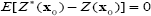
Kriging is a type of interpolation technique. The procedure is similar to averaging techniques of interpolation but the weights are derived from the spatial arrangement as well as from the distance between nearby points, i.e. from the variogram. The fitted variogram or the directional variogram (for anisotropic variation) is/are used to determine the weights λi needed for local interpolation. The weights are chosen so that the estimate is unbiased, and that the estimation variance is less than for any other linear combination of the observed values. Mapping the spatial distribution of a soil property involves interpolation or spatial prediction. Geostatistical interpolation uses the variogram to optimize prediction by kriging. The most basic form of kriging is ordinary punctual kriging in which the unknown value z(x0) of a given realization of Z(x0) in an unsampled point x0 is predicted from the known values z(xi) i= 1, 2, . . ., N, at the support points xi of the same realization using a so-called "best linear unbiased estimator" (BLUE). The best linear unbiased predictor z*(x0) of Z(x0) is given by a linear combination of the bservations:

Where λ, i are weights. The weights are chosen in such a way that the estimator is unbiased:

And the estimation is minimized.

Using a Lagrangian multiplier μ, minimization of the estimation variance under the constraint of unbiasedness yields a set of N+1 linear equations:

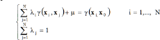
From which the and μ can be calculated. The estimation variance is then given by:

And represents the uncertainty in the prediction in x0. g (^xi, x^j) and g(xi, x 0) are the semi-variances between the observed locations xi and xj and between the observed location xi and the interpolated location x0, respectively. In the case of spatial dependence, semivariance tends to increase with the distance between observations; therefore errors decrease with the density of data and not just with their total number, as is the case with traditional statistical models. It needs to be pointed out that kriging is optimal and unbiased only on the condition that the model is correct. However, predictions are only slightly affected by the choice of the model, provided it is reasonable of course. This is one of the strengths of kriging that is robust enough in this sense; however, error variances can be seriously affected by the model Castrignanò [19].

Kriging has Many Useful Properties

a) The interpolated value is the most precise in terms of mean squared error

b) The interpolated value can be used with a degree of confidence, because an error term is calculated together with the estimation

c) The estimation variance depends only on the semi- variogram model and on the configuration of the data locations in relation to the interpolated point and not on the observed values themselves

d) The conditions of unbiasedness ensure that kriging is an exact interpolator, because the estimated values are identical to the observed values when a kriged location coincides with a sample location. In this case the weights within the neighbourhood are all zero and the estimation variance equals the observation.

e) Only the nearest few samples are spatially correlated to the kriged location and therefore they are the most weighted. Two important advantages become clear: firstly, the variogram needs to be accurate only in the first few lags; secondly whatever is gained from introducing distant points is limited also because sample locations interposed between the kriged point and more distant samples screen the distant ones by reducing their weights Castrignanò [19].

Validation Test

In geostatistical practice, the usual method of testing is crossvalidation. However, its results are actually biased and somewhat too optimistic Creutin and Obled [20], because it retains the same variogram, whereas the variogram should be recomputed and fitted every time that an observation is removed Laslett et al. [21]. Moreover, cross-validation is not true validation, because the same sample data set is used for both estimation and validation. All these shortcomings can be avoided by using a separate independent set of data for validation. So a validation data set consisting of 28 soil samples was used.

Prediction Assessment

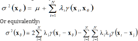
The performance of the prediction was assessed using cross validation Isaaks & Srivastava [22], whereby one observation (z) at a time is temporally removed from the data set and re-estimated (z*) from the remaining data. To assess the precision and accuracy of estimation of the soil variable under study, two statistical criteria were considered: mean error (ME), as an indicator of bias, and mean standardized squared error (MSSE) (scaled by the predicted standard deviation of estimation), as an accuracy measure:

Where N is the number of active observations and a the cokriging standard deviation, If the estimation is unbiased and accurate, the first statistic should be close to zero, where as the second one should be close to one, because the latter corresponds to the ratio between an experimental variance and a theoretical one Carroll & Cressie [23].

Calculations of leaching requirements for different delineated zones, Reclamation requirement was calculated using Reeve equation [24].

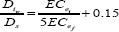
Where D_iw is the depth of leaching water (cm), Ds is the depth of soil (cm), EC_ei and EC_ef are soil salinity in dS m^-1 before and after leaching respectively. Leaching requirement was calculated to reduce soil salinity to be 2 dS m^-1 for only zones having a mean value of ECe higher than 4 dS.m^-1 for 0.20m depth. The mean value and area of each delineated zones were calculated as follows:

a) Reclassification of the interpolated raster map using "reclassify" tool, available in spatial analyst tools.

b) Applying of "raster to polygon" tool, available in conversion tools to convert a raster dataset to polygon features

c) Use of "dissolve" tool , available in data management tools to unify polygons of the same class based on grid code number

d) Use of "zonal statistics as table" tool, available in Spatial analyst tools to obtain the mean value of each class

e) Use of "calculate areas", available in spatial statistics tools to calculate the area of each class.

The leaching requirements was also calculated based on the average value of all samples (91) to quantify the water saved and make a good comparison between the two geostatistical and traditional methods.

Table 2 shows that the calibration and validation data sets were extracted from the same population since the p-value (0.06) is greater than a value (0.05) in the achieved t test. This is an important criterion to use different data set in validation (Table 2).

Table 2: Results of t test with unequal variances.

Table 3: Parameters of the fitted spherical variogram model.

Variogram Parameters

Table 3 and Figure 1 show variogram model parameters where a spherical model with nugget effect equal to 1.18 was fitted to the experimental variogram. The range of autocorrelation was 57.39 m and the partial sill was 1.60 (Table 3) & (Figure 1).

Prediction Assessment

Table 4 shows the assessment statistics in cross-validation and validation data sets. It can be seen that results of cross-validation are better than those of validation. However results of validation are more reliable. The mean error and MSSE in cross-validation and in validation were 0.09 and -0.95 and 1.07 and 1.27 respectively. Although the MSSE values is somewhat far from 1 but still within the tolerance interval (±3√2/N, N is number of observations) Chiles & Delfiner [25], which means that the model is accurate (Table 4). Table 5 shows the different quantities of water to be added to the soil to reduce soil salinity to 2 dS.m^-1 in the different classes (Figure 2). There is no need to leach the first class, named as low, whereas in the medium class, 3625m³ of water should be added to reduce the salinity in that area to reach 2 dS.m^-1. To reduce the salinity of the high class, 1149m³ of water should be added to reduce its salinity to 2 dS.m^-1. It is worth mentioning that assuming the ECe mean value for 91 soil samples (5.12 dS.m^-1) - without geostatistical interpolation - a quantity of 6203 m³ of water should be added to reduce salinity of the whole field to 2 dS.m^-1. So 1429 m³ can be saved and then used for irrigation [26,27]. These results emphasize the importance of geostatistical techniques in detecting within field variability and hence applying site-specific management (Table 5) & (Figure 2).

Figure 1: variogram model.

Figure 2: ECe spatial map interpolated by ordinary kriging, with mean value of each class.

Figure 3: Soil texture classes in some samples over the field.

Table 4: ME and MSSE in cross-validation and in validation data sets.

Table 5: Leaching requirements for delineated classes and all samples.

The low ECe values found in the south western area of the field whereas high and medium ECe values were observed in the remaining areas of the field, In order to interpret the reason beyond the existence of different areas with different ECe values, a quick check of soil texture (Figure 3) was performed to interpret the low, medium and high ECe values in the delineated zones. The results of soil texture proved that the low values coincided with the coarser soil texture (light clay) and then increased infiltration rate. The high and medium values detected in the remaining parts of the field coincided with heavier soil texture (heavy clay) (Figure 3).

Soil properties vary greatly over space and/or time. So it is necessary to recognize the spatial and temporal variation in soil properties. This cannot be achieved by the traditional methods based on averages of laboratory measured data and hence the essence of the usage of the developed tools such as geostatistics. Geostatistics allows predicting soil properties in unsampled locations and consequently to delineate site-specific management zones which are used for variable rate applications. In this study, a prescription map of leaching requirements was developed using ordinary kriging. The prediction map was classified into 3 management zones with different mean values of salinity. One of the three management zones had a mean value of ECe lower than 4 whereas the remaining two zones had ECe values higher than 4. So the leaching requirements were calculated only for zones having ECe higher than 4. A comparison between traditional method of calculating leaching requirements based on average of collected samples and geostatistical method was achieved and a quantity of 1429 m3 water was saved by applying the geostatistical method. These results encourage the use of geostatistics to develop site- specific management zones for leaching requirements especially in arid and semi arid regions and under water scarcity conditions.

1. Eilers RG, Eilers WD, Fitzgerald MM (1997) A salinity risk index for soils of the Canadian Prairies. Hydrogeology Journal 5(1): 68-79.
2. Herrero J, Pe'rez-Coveta O (2005) Soil salinity changes over 24 years in a Mediterranean irrigated district. Geoderma 125(3-4): 287-308.
3. Benyamini Y, Mirlas V, Marish S, Gottesman M, Fizik E, et al. (2005) Agricultural Water Management 76(3): 181-194.
4. Wang LP (1998) Synthetic analysis for extracting information on soil salinity using remote sensing and GIS: A case study of Yanggao basin in China. Environmental Management 22(1): 153-159.
5. Amezketa E (2006) An integrated methodology for assessing soil salinization, a pre-condition for land desertification. Journal of Arid Environment 67(4): 594-606.
6. (2007) Land and plant nutrition management service. FAO.
7. 7.  Oliver MA, and Webster R (2015) Basic Steps in Geostatistics: The Variogram and Kriging. Springer Briefs in Agriculture.
8. Navarro Pedreno J, Jordan MM, Melendez Pastor I, Gomezi I, Juan P, et al. (2007) Estimation of soil salinity in semi-arid land using a geostatistical model. Land Degrad Develop 18: 339-353.
9. Burgess TM, Webster R (1980) Optimal interpolation and isarithmic mapping of soil properties: I The variogram and punctual kriging J Soil Sci 31(2): 315-331.
10. Warrick AW, Myer DE, Nielsen DR (1986) Geostatistics methods applied to soil science. In A. Klute (Eds.). methods of soil analyses part 1: Physical and mineralogical methods p. 53-82.
11. Odeh IOA, Mc Bratney AB, Chittleborough DJ (1992) Fuzzy-c means and kriging for mapping soil as continues system. Soil Sci Soc Am J 56: 18481854.
12. Juang KW, Lee DY (2000) Comparsion of three nonparametric kriging methods for delineating heavy-metal contaminated soils. J Environ Qual 29(1): 197-205.
13. Lopez Granados F, Jurado-Exposito M, Pena Barragan JM, Garcia Torres L (2015) Using geostatistical and remote sensing approaches for mapping soil properties. Eur J Agron 23: 279-289.
14. Meul M, Van Meirvenne M (2003) Kriging soil texture under different types of nonsationarity. Geoderma 112(3-4): 217-233.
15. Sumfleth K, Duttmann R (2008) Prediction of soil property distribution in paddy soil landscapes using terrain data and satellite information as indicators. Ecol Indic 8(5): 485-501.
16. Jackson ML (1973) Soil Chemical Analysis. Prentice Hall, Englewood Califfs, New Jersy, USA.
17. Slavich PG, Petterson GH (1993) Estimating the critical conductivity of saturated paste extracts from 1:5 soil: water suspensions and texture. Australian Journal of Soil Research p. 73-81.
18. Moeys J (2016) the soil texture wizard: R-functions for plotting, classifying transforming and exploring soil texture data. Swedish Univ of Agriculture Sci, Uppsala, Sweden.
19. Castrignano A (2011) Introduction to spatial data analysis. Aracne, Rome.
20. Creutin J, Obled C (1982) Objective analysis and mapping techniques for rainfall fields. An objective comparison. Water Resource Research 18: 413-431.
21. Laslett GM, McBrathney AB, Pahl PJ, Hutchison MF (1987) Comparison of several spatial methods for soil pH. Journal of Soil Science 38: 325341.
22. Isaaks EH, Srivastava RM (1989) An Introduction to Applied Geostatistics. Oxford University Press pp. 561.
23. Carroll SS, Cressie N (1996) A comparison of geostatistical methodologies used to estimate snow water equivalent. Journal of the American Water Resources Association 32(2): 267-278.
24. Reeve RC (1975) the relation of salinity to irrigation and drainage requirement. 3^rd Cong on Irrigation and Drainage Tran 5: 157-187.
25. Chiles JP, Delfiner P (1999) Geostatistics: Modelling Spatial Uncertainty.Wiley, New York, USA, pp. 695.
26. (1993) Soil Survey Division Staff 1993, Soil survey manual. Soil Conservation Service. Department of Agriculture Handbook, USA.
27. Webster R, Oliver MA (2007) Geostatistics for environmental scientists. (2^nd edn) John Wiley & Sons, Ltd, USA.