Understanding the Connections between Inexact Newton-Krylov PDE-Constrained LDDMM and LDDMM via Geodesic Shooting and Efficient Adjoint Calculation Volume 4 - Issue 1

Monica Hernandez*

• Computer Sciences Department, Aragon Institute on Engineering Research (I3A), University of Zaragoza, Spain

Received: February 02, 2018;   Published: April 23, 2018

*Corresponding author: Monica Hernandez, Computer Sciences Department, Aragon Institute on Engineering Research (I3A), University of Zaragoza, Spain

DOI: 10.26717/BJSTR.2018.04.000990

Abstract PDF

This work studies the connections between two PDE-constrained diffeomor-phic registration methods. The methods have been selected for their relevance in the diffeomorphic registration literature. From the initial PDE-constrained variational formulation, the methods seem to be highly unrelated. However, an in-depth study of the derivations involved in the computation of the optimiza-tion ingredients reveals interesting connections that are worth to be stated. The insights provided in this work may bridge the gap between both methods, underpinning the proposal of improved PDE-constrained LDDMM methods.

Deformable image registration is the process of computing spatial transforma-tions between different images so that corresponding points represent the same anatomical location. There exists a vast literature on deformable image registrations methods with differences on the transformation characterization, regularizes, image similarity metrics, optimization methods, and additional con-straints [1]. In the last two decades, diffeomorphic registration has arisen as powerful paradigm for deformable image registration [2]. Diffeomorphisms (i.e., smooth and invertible transformations) have become fundamental inputs in Computational Anatomy. There exist different big families of diffeomorphic registration methods. In this work, we focus on PDE-constrained diffeomorphic registration method due to its relevance in the last decade. PDE-constrained diffeomorphic registration augments the original variational formulation with Partial Differential Equations (PDEs) of interest. The firs Preprint submitted to Biomedical Journal of Scientific and Technical research March 28, 20 methods was proposed by Hart et al. [3].

In that work, the problem was for-mulated as a PDE-constrained control problem subject to the state PDE and the relationship with Beg et al. LDDMM [4] was stated. Later on, Vialard et al. proposed a PDE-constrained method parameterized on the initial momen-tum [5]. More recently, Mang et al. have proposed a PDE-constrained method that extended the gradient-descent optimization in Hart et al. approach to in-exact Newton-Krylov optimization [6]. Our attention is focused on the last two methods since, in our opinion; they constitute milestones on PDE-constrained LDDMM. From the formulation and the notation used in [5] and [6] one may think that both methods are highly unrelated. However, from an in-depth study of the derivations involved in the computation of the gradient and the Hessian-vector products in the design of the corresponding optimization methods, one can realize that both methods are quite related. This work studies the connections between both methods. We revisit both methods and rewrite the equations adopting the same notation for the corresponding variables. In the end, we analyze the simi-larities between both methods. We believe that the insights provided in this work may bridge the gap between both methods and help to build improved PDE-constrained diffeomorphic registration methods.

Background on LDDMM

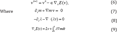
In this section, we introduce the notation and the fundamental ideas underpin-ning the Large Deformation Diffeomorphic Metric Mapping (LDDMM) paradigm as proposed by Beg et al. [4]. We consider images defined on the image domain Ω⊆R^d, d = 2, 3. We denote with Diff(Ω) to the Riemannian manifold of diffeo-morphisms on Ω. We denote with V to the space of smooth vector fields on Ω. V is the tangent space of the Riemannian structure at the identity diffeomorphism, id. The right composition of diffeomorphisms endows Dif f (Ω) with a Lie group structure, where V is the corresponding Lie algebra. The right-invariant Riemannian metric is defined from the scalar product

Where is the invertible self-adjoint differential operator associated with the differential structure of Dif (Ω) . In the following, the inverse of the operator L will be denoted by K. Let I0, and I1 be the source and the target images defined on Ω. The LDDMM variational problem is given by the minimization of the energy functional

In contrast to traditional non-rigid image registration, the problem is posed in the space of time-varying smooth flows of velocity fields in This allows obtaining deformations larger than conventional approaches posed in the space of displacement fields. Given the smooth flow the diffeomorphism φ^v ₁ is defined as the solution at time 1 to the transport equation

With initial condition φ₀^v = id. The transformation(φ₁^v )¹ computed from the minimum of E (v) is the diffeomorphism that solves the LDDMM registration problem between I0 and I1. The optimization of Equation (2) was originally approached using gradient-descent in More recently, optimization has been approached using Gauss-Newton methods [7].

Inexact Newton-Krylov PDE-constrained LDDMM

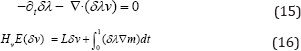
PDE-constrained LDDMM method was originally proposed by Hart et al. in [3]. Departing from LDDMM variational problem, PDE- constrained LDDMM is given by the minimization of

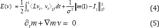
With initial condition m(o) = I₀. The variable m represents the evolution ofl₀o(φ₁^v)^-1 under the transport equation, although, numerically, the solution of the state equation and the evolution of the composition yield different results. This quantity is called the state variable, and Equation (5) is referred as the state equation. The velocity v is referred as the control variable. The optimization of this problem has been approached using gradient-descent [3] and inexact Newton-Krylov methods [6]. The gradient-descent update equation is obtained from

With initial conditions 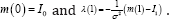Equation [8] is the adjoint equation and λ is referred as the adjoint variable. The quantity is referred as the body force. While the state equation is solved forward (i.e. starting from t = 0), the adjoint equation is solved backward (i.e. starting from t= 1). Inexact Newton-Krylov optimization is implemented using Preconditioned Conjugate Gradient (PCG), yielding to the update equation

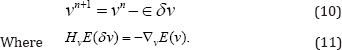
The Hessian-vector product H_vE (δv) is computed from the incremental equations associated to the state, adjoint, and gradient expressions. Thus,

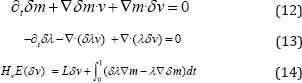
One important concern in the design of practical Newton methods is to keep the computational cost as small as possible. Inexact Newton methods achieve this objective by terminating PCG before an exact solution is found. Therefore, inex-act Newton-Krylov optimization computes an approximation of the pure Newton step in each iteration. It should be noticed that the Hessian can be indefinite or singular far away from the solution. In these cases, the search directions computed in PCG may not be descending directions. Therefore a Gauss-Newton approximation of the expression of H_vE (δv) is used in practice. Thus, the incremental adjoint variable and the Hessian-vector products are computed from

The optimization approach can be classified as a reduced space method. Al-though the problem depends on the state, adjoint, and control variables, the iterations are performed only on the reduced space of the velocity field (the con-trol variable). With this approach, we should assume that the state and adjoint equations are fulfilled exactly. Therefore, for the computation of the gradient and the Hessian-vector products the state and adjoint equations and their incremental counterparts need to be solved. For accepting a numerical solution as optimal, the reduced gradient should be close to zero. The method is combined with important numerical implementation approaches. As most remarkable, a Galerkin representation is used for the parameterization of the time-varying velocity fields and spectral methods are used for differentiation, ODE integration, and time integral computation. We refer to the excellent work by Mang et al. for the details [6].

LDDMM via geodesic shooting and efficient adjoint calculation

LDDMM via geodesic shooting and efficient adjoint calculation was proposed by Vialard et al. [5]. The problem is formulated from the minimization of

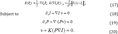
The problem is posed on the initial adjoint variable constrained with the state and adjoint equations. Both equations are solved in the forward direction. The variable I represents the state variable while P represents the adjoint variable. The control variable equation comes from the momentum conservation equation in metamorphosis [8]. From the control equation, the regularization energy is encoded using the norm of the initial momentum

Therefore, this method can be classified as a PDE-constrained LDDMM method based on geodesic shooting. In the following, this method will be recalled as GS PDE-constrained LDDMM. The optimization of this problem has been approached using gradient- descent. The update equation is obtained from

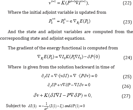
This optimization approach can also be classified as a reduced space method. Instead of reducing the computations to the optimization in the space V, the optimization is reduced to the space of initial adjoint variables. The method uses finite differences for the computation of the derivatives. In-stead of solving the state and adjoint equations and their incremental counter-parts, the authors proposed to solve the transport equation and compute I from and P from . Second-order time integration methods such as Min-Mod or Super Bee limiters were considered in the solution of the transport equation.

Establishing Connections

In order to establish the connections between PDE-constrained LDDMM and GS PDE-constrained LDDMM, we rewrite GS PDE- constrained LDDMM using the notation of [6]. To this end, the state variable I will be replaced by m, and the adjoint variable P will be replaced by-λ . In addition, the incremental state variable δP will be replaced by δm, the incremental adjoint variable δI will be replaced by δλ , and the incremental control variable δv will be replaced by -δv . (Tables 1-3) gather the equivalent equations of both methods using this notation. Table 1 gathers the equations associated with the problem formulations. While PDE-LDDMM is posed on the space of time-varying velocity fields, GS PDE-LDDMM is posed on the space of initial adjoint variables. Both problems can be identified as reduced-space methods. However, the reduced spaces where optimiza-tion is performed are different for both approaches. PDE-LDDMM is constrained using a single PDE while GS PDE-LDDMM is constrained using two PDEs and a single equation on the control variable. The control equation identifies with the momentum Lv the body force derived for the gradient in PDE-LDDMM.

Table 1: Problem formulation equations.

PDE-constrained problems

At first sight, both problems seem quite different in their original formulation. However, in Table 2 it can be appreciated that both methods solve the same state and adjoint equations. The only difference is that the adjoint equation is solved backward with initial condition λ₀ⁿ with λ_o^o = 0. Even more, in Table 3 it can be appreciated that both methods solve the same incremental state and adjoint equations. The differences come from the direction of the incremental state equation (backward for GS PDE-LDDMM) and the initial condition of the incremental adjoint equation (equal to the initial condition of the adjoint equation in PDE-LDDMM). The incremental control equation identifies with the incremental body force derived for the Hessian in PDE-LDDMM.

Table 2: First-order equations.

State and Adjoint equations. Gradient and control.

Table 3: Second-order equations.

Incremental state and adjoint equations. Hessian and incremental control.

Figure 1: RMSE convergence curves of PDE-LDDMM with the stationary and the non-stationary parameterization, and GS PDE-LDDMM. The curves relative to Gauss-Newton-Krylov optimization have been corrected for the number of PCG inner iterations.

Figure 2: Image registration results. Sagittal view of the warped sources (left), image differences after registration (center), and the initial velocity fields v0 (right).

In this section, we compare the performance of PDE-LDDMM and GS PDE-LDDMM. The experiments were conducted on a representative dataset from the NIREP [9]. The computations were performed on an NVidia GeForce GTX 1080 ti with 11 GBS of VRAM and an Intel Core i7 computer with 32 GBS of DDR3 RAM. Due to memory issues, the images were resampled into volumes of size 90 x 105 x 90. Figure 1 shows the convergence curves of the image similarity error relative to the first iteration The pslot shows that the convergence rate of inexact Gauss-Newton-Krylov PDE-LDDMM is extraordinarily fast in comparison with the convergence of gradient-descent optimization used in GS PDE-LDDMM. The convergence curve of PDE-LDDMM with the non-stationary parameterization slightly over passed the stationary parameterization. Figure 2 shows the registration results for a qualitative assessment of the methods.

In this work, we have studied the connections between two apparently unrelated PDE-constrained diffeomorphic registration methods. We have shown that both methods are based on the same PDEs with differences in the integration direction and the initial condition of the adjoint and the incremental adjoint equations. The different initial conditions come from including the adjoint equation as a constraint of the problem in the geodesic-shooting approach. The control and the incremental control in geodesic-shooting are related to the body force and the incremental body force arising in the gradient and Hessian-product expressions associated with the control variable. Inexact Newton-Krylov optimization shows an excellent numerical accuracy and an extraordinarily fast convergence rate in PDE-LDDMM.

However, diffeo-morphism parameterization is restricted to the Galerkin representation of the stationary and non-stationary velocity fields. The most interesting feature of GS PDE-LDDMM is the parameterization in the space of initial momenta. However, the optimization approach based on gradient-descent yields a slow convergence rate, even though the incremental equations are used in the computations. As future work, we believe that it would be interesting to use the equations from GS PDE-LDDMM in the inexact Newton-Krylov optimization framework of PDE-LDDMM towards a method parameterized with the initial momentum. It would also be interesting to compare the performance of reduced methods on the space of initial controls vs initial adjoins. Furthermore, future methods would benefit from using spectral methods [10] in the numerical computations.

The author would like to acknowledge the national research grant TIN2016-80347-R.

1. Sotiras C, Davatzikos, N Paragios (2013) Deformable medical image registration: A survey, IEEE Trans. Med. Imaging 32(7): 1153-1190.
2. MI Miller (2004) Computational anatomy: shape, growth, and atrophy comparison via diffeomorphisms, Neuroimage 23(suppl 1): 19-33.
3. GL Hart, C Zach, M Niethammer An optimal control approach for deformable registration.
4. MF Beg, MI Miller, A Trouve, L Younes (2005) Computing large deformation metric mappings via geodesic flows of diffeomorphisms, Int J Comput Vision 61(2): 139-157.
5. FX Vialard, L Risser, D Rueckert, DD Holm (2012) Diffeomorphic atlas estimation using geodesic shooting on volumetric images, Annals of the BMVA 2012(5): 1-12.
6. A Mang, G Biros (2015) An inexact Newton-Krylov algorithm for constrained diffeomorphic image registration, SIAM J Imaging Sciences 8(2): 1030-1069.
7. M Hernandez, Gauss-Newton inspired preconditioned optimization in large deformation diffeomorphic metric mapping, Phys. in Med. and Biol 59(20): 6085-6115.
8. DD Holm, A Trouve, L Younes (2010) The Euler-Poincare theory of metamorphosis. Q Appl Math 67(4).
9. JH Song, GE Christensen, JA Hawley, Y Wei, JG Kuhl (2010) Evaluating image registration using NIREP, pp: 140-150.
10. LN Trefethen Spectral methods in matlab, SIAM, Philadelphia.