Restricted Boltzmann Machine and its Potential to Better Predict Cancer Survival Volume 6 - Issue 1

Ruibang Luo*, Wen Ma and Tak-Wah Lam

• Department of Computer Science, The University of Hong Kong, China

Received: June 20, 2018;   Published: June 26, 2018

*Corresponding author: Dr. Ruibang Luo, Assistant Professor, Department of Computer Science, The University of Hong Kong, Pokfulam Road

DOI: 10.26717/BJSTR.2018.06.001305

Abstract PDF

Traditional methods to predict cancer survival include Competing-Risk Regression and Cox Proportional Hazards Regression; both require the hazard of input variables to be proportionate, limiting the use of non-proportionate measurements on miRNA inhibitors and inflammatory cytokines. They also require imputation at missing data before prediction, adding fallible workloads to the clinical practitioners. To get around the two requirements, we applied Restricted Boltzmann Machine (RBM) to two patient datasets including the NCCTG lung cancer dataset (228 patients, 7 clinicopathological variables) and the TCGA Glioblastoma (GBM) miRNA sequencing dataset (211 patients, 533 mRNA measurements) to predict the 5-year survival. RBM has achieved a c-statistic of 0.989 and 0.826 on the two datasets, outperforming Cox Proportional Hazards Regression that achieved 0.900 and 0.613, respectively.

Abbrevations: RBM: Restricted Boltzmann Machine; GBM: Glioblastoma; AFP: Alpha-Fetoprotein; AUC: Area Under The Curve

The rapid development of new computational methods and tools for data analysis and building predictive models has enabled more precise cancer prognosis. Use the prediction of the risk of recurrence after liver transplantation as an example, in the recent years, researchers and clinical practitioners have discovered several clinicopathological variables that play an important role, such as the number and size of tumors and the level of alpha-fetoprotein (AFP). There were a few significant studies of patients who underwent primary liver transplantation; to name a few, Mazzaferro et al. [1] studied a cohort of 1,018 patients at three tertiary centers in Italy and achieved an average c-statistic of 0.780 on predicting 5-year risk of HCC-related death using 2 variables including:

a) Sum of tumor number and size and

b) Logarithmic level of AFP.

Ling et al. [2] studied a cohort of 1,010 patients extracted from the China Liver Transplant Registry database and achieved a c-statistic of 0.767 on predicting 2-year risk of HCC recurrence using 4 variables including:

a) Cold Ischemia Time,

b) Tumor Burden,

c) Differentiation And

d) Afp.

Mehta et al. [3] studied a cohort of 1,061 patients at 3 academic transplant centers including the University of California-San Francisco; Mayo Clinic, Rochester; and Mayo Clinic, Jacksonville, and achieved a c-statistic of 0.82 on predicting 5-year risk of HCC recurrence using 3 variables including:

a) Micro Vascular Invasion

b) Afp and

c) The sum of the Largest Viable Tumor Diameter and Number of Viable Tumors on Explant.

Agopian et al. [4] studied a cohort of 865 patients at University of California, Los Angeles from 1984 to 2013 and achieved a c-statistic of 0.85 on predicting 5-year risk of HCC recurrence using 8 variables including:

a) Nuclear Grade,

b) Macrovascular Invasion,

c) Milan Criteria,

d) Nonincidental and Radiologic Maximum Diameter

e) Microvascular Invasion,

f) Neutrophil-Lymphocyte Ratio,

g) Afp and

h) Total Cholesterol.

The first study is using Competing-Risks Regression, while the second, third and fourth studies are using Cox Proportional-Hazards Regression to analyze the impact of potential factors on patients’ recurrence or survival. With Competing-Risks Regression, one focuses on the cumulative incidence function that indicates the probability of the event of interest happens before a certain time, while in Cox Proportional Hazards Regression, one instead focuses on the survival function that indicates the probability or survival beyond a certain time. Although both the Competing-Risk Regression and Cox Proportional Hazards Regression method have been widely adopted in biomedical research for investigating the association between the recurrence time and survival time of patients and one or more predictor variables, there are requirements to satisfy for the two methods to work correctly

One requirement is the proportionality of the hazard of the input variables. That is, using variables that might strengthen or weaken as a hazard factor of recurrence along the time in the two regression methods may result in a false inference. In practice, only some but not all variables satisfy this requirement [5]. Moreover, this limits the use of variables with a time-varying effect such as the circulating proteins (e.g., the level of some inflammatory cytokines), or transcriptome profile (e.g., the abundance of some miRNA inhibitors) to enhance the prediction performance. According to the previous studies, the c-statistic is higher when using more variables (say, 0.85 using 8 variables against 0.82 using 3 variables). Hence, a computational method that allows variables with unproportionate hazards along the time is needed. Another requirement of the two regression methods is that there must be no missing data, i.e., as not all the variables were measured for all the patients, either we reduce the number of patient samples to fulfill a broader set of usable variables, or we use a smaller set of variables to increase the number of usable patient samples. A common practice to alleviate the downside of missing data is to do multiple imputation before prediction [6]. However, multiple imputation is computationally intensive. Some algorithms need to be run multiple rounds to get the approximation, and the required runtime increases when more data are missing [7]. Moreover, it adds additional workloads to the clinical practitioners to learn not only how to do multiple imputation, but also how to identify possible imputation failures to avoid a “garbage in, garbage out” situation in the following prediction.

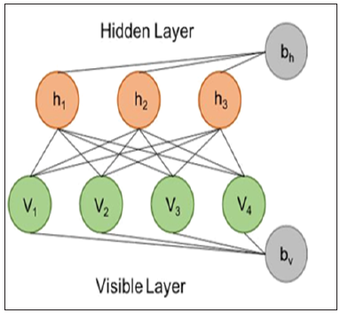
To get around the two requirements, in our study, we leveraged the power of Restricted Boltzmann Machine (RBM) for both the problem of missing data imputation and the problem of post-transplantation recurrence risk prediction. RBM is an undirected, probabilistic and parameterized neural network model (Figure 1). Although RBM has one of the simplest architectures of all neural networks, it is often used amongst other machine learning methods to extract vital information from an unknown distribution of some high-dimensional data. RBM captures dependencies between variables by associating an energy to each configuration of the variables and the training of RBM is basically finding a combination of parameters for the given input values so that the sum of energies reaches a minimum. Imputation using RBM works by clamping the value of the observed variables and finding configurations of the missing variables that minimize the energy. A detailed guide to training and using RBM were made available by Hinton et al. [8]. Previous studies have estimated RBM’s power in imputing high-dimensional datasets [9,10]. RBM has been successfully applied to imputing acoustic speech signal [11], but its power on imputing biomedical data has not been studied. In our study, we provided a best-practice and filled the gap of using RBM on biomedical data. Specifically, we modeled the risk prediction problem as an imputation problem by feeding in the known risk of post-translation recurrence during model training, and intentionally leave the risk blank (or more precisely, fill in a random value Gibbs sampled from its exact conditional distribution) when making inference from a trained model. We used the RBM model implementation publicly available at the link “https://github.com/Cospel/rbm-ae-tf”. The code was written in Python using a popular machine learning platform named Tensorflow, and can be modified easily. We changed the number of input nodes in the code to fit our data. We also increased the number of hidden nodes to 50 in order to increase the model’s power to learn the nonlinearity and multicollinearity of the input variables, although it takes longer and more computational resources to train the model. Sigmoid was used as the activation function between the visible (input) layer and the hidden layer. In terms of hyperparameter tuning, we used the Adam optimization algorithm with an initial learning rate at 0.001 as the stochastic optimization method to train the RBM. A sparsity penalty the same as the value of learning rate was applied to the training. L2 regularization (weight-decay) was also applied to avoid model overfitting with the lambda set to 0.9 times the sparsity penalty. We randomized the order of the training samples and used 64 samples as the batch size. We held out 20% of the input samples as the validation data, and we stopped the model training when a higher scalar energy is observed in the validation data than the training data for continuously 5 epochs. We initiated the weights of the model with small random values chosen from a zero-mean normal distribution with a standard deviation of 0.01. We also initiated the biases to log $’(%%&&), where pi is the proportion of training samples in which the value is non-zero. To test the power of our RBM model, we first used the NCCTG lung cancer dataset [12] that contains 228 patients and 7 clinicopathological variables. The dataset is freely available and was provided as a part of the “survival” package in the R programming language. Besides the institution code, survival time in days and the patients’ vital status, the dataset contains 7 clinicopathology variables for building a model to predict the 5-year survival rate. The variables include:

a. Age

b. Sex

c. ECOG performance score

d. Karnofsky performance score rated by physician

e. Karnofsky performance score rated by patient

f. Calories consumed at meals and

g. Weight loss in last six months.

Figure 1: An RBM model consists of a visible (input) layer with four nodes and a hidden layer with three nodes, and the corresponding biases vector for both layers.

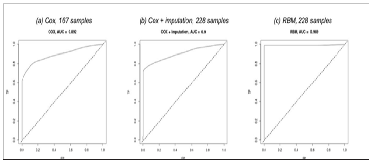
The dataset has 167 (73.25%) patients with all variables available, and the remainder is with one or more missing variables (Figure 2). We first studied the performance of the traditional Cox Proportional Hazards Regression on the 167 patients by building models for ten groups of samples, each group generated by randomly dividing the patients into 80% for model training and 20% for evaluating the c-statistic (also named as AUC, the Area Under the Curve). The ten trained models have achieved an average c-statistic of 0.892 (Figure 3a). Next, in order to increase the number of usable patients for building a model, we imputed the dataset using the “mice” package in R with the “Predictive Mean Matching” algorithm. The algorithm by default have generated five imputed datasets and we picked the second in our study. We also built ten Cox regression models on the imputed dataset with 228 patients and achieved an average c-statistic of 0.900 (Figure 3b), which is slightly higher than without imputation. Then we worked on training RBM models. The training of the RBM model used less than a minute on a nVidia GTX1080 GPU and won’t exceed a couple of minutes using a multi-core general CPU. For those patients with missing data, we used different numbers of visible (input) nodes in the model, while the number of hidden nodes remained the same. To make inference from the trained RBM model, we feed the model with

Figure 2: The summary of missing data in the NCCTG lung cancer dataset.

Figure 3: The Receiver Operating Characteristic (ROC) curve and the c-statistic (AUC) of the three different methods on the NCCTG lung cancer dataset.

a. Known variables;

b. Missing variables in the visible (input) layer, each substituted by a random value Gibbs sampled from the exact conditional distribution of that variable, and

c. The probability of recurrence with 0 as the initial value.

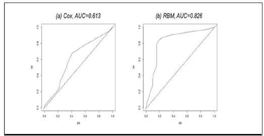
After input, the RBM model was iterated for 500 steps to burn in, and we define recurrence probability >0.5 as recurrent. We also trained ten RBM models on ten groups of samples. The models achieved an outstanding average c-statistic of 0.989 (Figure 3c). Then, we tested RBM’s power in dealing with non-proportionate data. We worked on the TCGA Glioblastoma (GBM) miRNA sequencing dataset with 211 patients and 533 miRNA measurements to predict the patients’ 5-year survival [13]. The dataset is publicly available at link https://www.synapse.org/#!Synapse:syn1710282. The survival time in days and the patients’ vital status are in the file with identifier “syn1710370”. The 533 miRNA measurements are available in the file with identifier “syn17103768”. We also built ten models using Cox Regression and RBM, respectively. The average c-statistic of using RBM is 0.826 (Figure 4b), which significantly outperformed Cox Regression (Figure 4a).

Figure 4: The ROC curve and the AUC of the two different methods on the TCGA Glioblastoma miRNA sequencing dataset.

In our study, we explored using RBM on biomedical data to allow missing variable and the hazard of input variables to be non-proportionate. Instead of doing imputation and prediction in separated steps, RBM integrates the two steps together by modeling the prediction as an imputation problem. The experiment on predicting the 5-year survival rate of 228 patients with 7 clinical pathological variables has shown that RBM model has achieved superior c-statistic on the raw data over using the traditional Cox Proportional Hazards Regression with imputed data. The experiment on predicting the 5-year survival rate of 211 patients with 533 mRNA measurements has shown that RBM surpassed the traditional method in dealing with a large amount of non-proportionate input variables.

1. Mazzaferro V, Sposito C, Zhou J, Pinna AD, De Carlis L, et al. (2018) Metroticket 2.0 Model for Analysis of Competing Risks of Death After Liver Transplantation for Hepatocellular Carcinoma. Gastroenterology 154(1): 128-139.
2. Ling Q, Liu J, Zhuo J, Zhuang R, Huang H, et al. (2018) Development of models to predict early post-transplant recurrence of hepatocellular carcinoma that also integrate the quality and characteristics of the liver graft: A national registry study in China. Surgery pii: S0039- 6060(18)30079-30075.
3. Mehta N, Heimbach J, Harnois DM, Sapisochin G, Dodge JL, et al. (2017) Validation of a Risk Estimation of Tumor Recurrence After Transplant (RETREAT) Score for Hepatocellular Carcinoma Recurrence After Liver Transplant. JAMA Oncology 3(4): 493-500.
4. Agopian VG, Harlander-Locke M, Zarrinpar A, Kaldas FM, Farmer DG, et al. (2015) A novel prognostic nomogram accurately predicts hepatocellular carcinoma recurrence after liver transplantation: analysis of 865 consecutive liver transplant recipients. J Am Coll Surg 220(4): 416-427.
5. Babińska M, Chudek J, Chełmecka E, Janik M, Klimek K, et al. (2015) Limitations of Cox Proportional Hazards Analysis in Mortality Prediction of Patients with Acute Coronary Syndrome 43(1): 33-48.
6. Janssen KJM, Vergouwe Y, Donders ART, Harrell FE, Chen Q, et al. (2009) Dealing with Missing Predictor Values When Applying Clinical Prediction Models. Clinical Chemistry 55(5): 994-1001.
7. Sterne JA, White IR, Carlin JB, Spratt M, Royston P, et al. (2009) Multiple imputation for missing data in epidemiological and clinical research: potential and pitfalls. Bmj 338: b2393.
8. Hinton GE (2012) A practical guide to training restricted Boltzmann machines. In Neural networks: Tricks of the trade. Springer, pp. 599-619.
9. Leke C, Marwala T (2016) Missing data estimation in high-dimensional datasets: a swarm intelligence-deep neural network approach. In International Conference in Swarm Intelligence. Springer pp. 259-270.
10. Leke C, Marwala T, Paul S (2015) Proposition of a Theoretical Model for Missing Data Imputation using Deep Learning and Evolutionary Algorithms. arXiv: 151201362.
11. Deng L, Li J, Huang JT, Yao K, Yu D, et al. (2013) Recent advances in deep learning for speech research at Microsoft. In Acoustics, Speech and Signal Processing (ICASSP), 2013 IEEE International Conference: IEEE 8604-8608.
12. Loprinzi CL, Laurie JA, Wieand HS, Krook JE, Novotny PJ, et al. (1994) Prospective evaluation of prognostic variables from patient-completed questionnaires. North Central Cancer Treatment Group. Journal of Clinical Oncology 12(3): 601-607.
13. Yuan Y, Van Allen EM, Omberg L, Wagle N, Amin Mansour A, et al. Assessing the clinical utility of cancer genomic and proteomic data across tumor types. Nature biotec 32(7): 644-652.