info@biomedres.us
+1 (502) 904-2126
One Westbrook Corporate Center, Suite 300, Westchester, IL 60154, USA
Site Map

Received: January 17, 2019; Published: January 29, 2019
*Corresponding author: Luis Gavete, Universidad Politécnica de Madrid, Spain
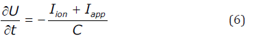
DOI: 10.26717/BJSTR.2019.13.002454


In this paper we present a fast, accurate and conditionally stable algorithm to solve a monodomain model in 2D, which describes the electrical activity in the heart. The model consists of a parabolic anisotropic Partial Differential Equation (PDE), which is coupled to systems of Ordinary Differential Equations (ODEs) describing electrochemical reactions in the cardiac cells. The resulting system is challenging to solve numerically, because of its complexity. We propose a simple method based on operator splitting and an explicit meshless method for solving the PDE together with an adaptive method for solving the system of ODE’s for the membrane and ionic currents.
Keywords: Electro Cardiology; Meshless; Monodomain; Generalized Finite Difference
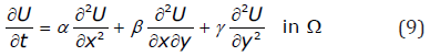
The obvious difficulty of performing direct measurements in electro cardiology has motivated wide interest in the numerical simulation of cardiac models. In this paper we will present a numerical scheme for the equations of the monodomain model, which describes the electrical activity in the heart. The approach presented herein including the use of a meshless method differs to the best of our knowledge from other numerical approaches in the literature. An operator-splitting algorithm [1] is used to split the monodomain model into PDE and systems of ODEs. Because of the irregular geometry of the cardiac muscle we use an Generalized Finite Difference Method (GFDM) for spatial discretization of the PDE together with an explicit method for time discretization. The explicit method includes a stability limit formulated for the case of irregular clouds of nodes that can be easily calculated.
The GFDM is evolved from classical Finite Difference Method (FDM). However, GFDM can be applied over general or irregular clouds of points. The basic idea is to use Moving Least Squares (MLS) approximation to obtain explicit difference formulae which can be included in the Partial Differential Equations. Benito, Ureña and Gavete have made interesting contributions to the development of this method [2,3,4]. In [5] the extension of the GFDM to the solution of anisotropic elliptic and parabolic equations is given. In [6] an FDM is presented to solve the bidomain equations. Althought this method is referred as a GFD scheme it is derived from a Taylor series expansion and a classic Least Squares (LS) method solved by a Moore-Penrose pseudo-inverse method together with a singular value decomposition method. This LS-GFDM uses elements to determine the nodal support templates. In our method a Taylor series expansion is used but the GFD scheme is obtained using Moving Least Squares (MLS) approximation. Then, the explicit difference formulae for irregular clouds of points can be easily obtained using a simple Cholesky method.
As the generalized finite difference approximation must be obtained at each point the approximations of the partial derivatives obtained by a local approximation (MLS) are much more accurate that those obtained by a global approximation (LS), see for example [7]. The MLS-GFDM is a truly mesh-free method using only points to determine the nodal supports. The main contribution of this paper is the application of an explicit scheme based in the MLS-GFDM to the case of modelling monodomain electrical conductivity problems using operator splitting including the case of anisotropic real tissues. The remainder of this paper is organized as follows. In Section 2 the monodomain model of cardiac tissue is introduced. In Section 3 we present how the monodomain model may be solved with an operator splitting method. In Section 4 the explicit GFDM is developed. Numerical experiments intended to validate the solution algorithm are presented in Section 5. Finally, in Section 6 some conclusions that can be drawn from the paper about the proposed method.
Mathematical models of cardiac electrophysiology consist of a system of Partial Differential Equations (PDEs), referred to as the bidomain model, coupled nonlinearly to a system of Ordinary Differential Equations (ODEs) modeling the membrane dynamics. Numerically, this system is challenging, and it is therefore common to seek possible simplifications. Simplifications can be derived either by reducing the complexity of the ODEs or the PDEs. The ODEs can be significantly simplified by using models of the cell membranes as model of FitzHugh-Nagumo type [8,9]. Furthermore, the bidomain model can be reduced from a system of two PDEs to a scalar PDE referred to as the monodomain model. An obvious advantage of monodomain models is their numerical efficiency: in some cases, monodomain models can be ten or more times faster for simulation of the same problem compared to bidomain models [10]. For simulation of wave propagation in the heart, monodomain models reproduce many of the phenomena that are observed experimentally and are thus an appropriate tool. Monodomain models are the focus of the present article
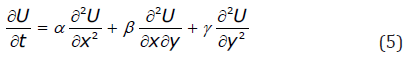
The monodomain approach assumes that cardiac tissue behaves as an excitable medium, with diffusion and local excitation of membrane voltage. It provides the simplest description of action potential propagation defined by the PDE:

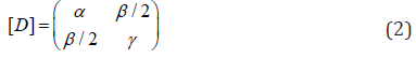
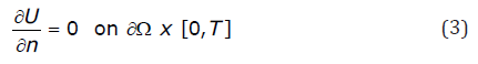
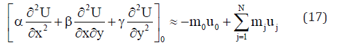
where α,β,γ are positive coefficients defining the conductivities of the anisotropic tensor [D] that describe the effective diffusion of voltage through the medium , C is membrane capacitance, U is local membrane potential, Iion is the total ionic current density (the flow of positive ions from inside to outside the cell through the membrane), and Iapp is any applied stimulus. Non-flux boundary conditions are used for two-dimensional tissue model simulations. Iion is a function of voltage U. Because of the fibrous structure of the heart muscle, the conductivity properties of the tissue are anisotropic. Typically, the conductivities in the direction along the muscle fibers will be higher than in the cross-fiber direction. Cardiac tissue anisotropy in monodomain models is given by the diffusion tensor [D] (related to conductivity by Eq. (2)), which can be found easily from the fiber direction and orientation of the sheet plane as was discussed for 2D in more detail in [5].
Monodomain models utilize zero flux boundary conditions, representing an isolated piece of cardiac tissue:
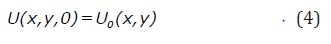
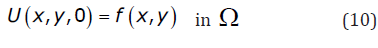
and impose initial conditions:
The general monodomain model can be expressed as a coupled system of a parabolic PDE and a system of ODE’s for the evolution of the local gating variable, that is a reaction-diffusion equation. In this paper we use an accurate Strang [1] splitting technique for a monodomain model, to separate the cell model ODEs from the PDE. The Strang splitting technique introduced in [11] will be used to separate the ODE system from the PDE, and the remaining PDE is discretized with an explicit GFD scheme. The algorithm has three steps:
Step 1) Use the result at time I as the initial condition to integrate the following PDE:
for a step length Dt/2 .
Step 2) Use the results of Step 1 as the initial condition to integrate the following ordinary differential equations (ODE’s):
where C and Iapp (t) are known In this Step, we integrate the cell model ODE’s for a time step Dt by using a modified FitzHugh- Nagumo model [13], given by
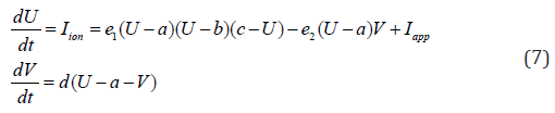
where a,b,c,d,e1,e2,… are constants.
The time step for solving the cell model ODEs (7) using fourth order Runge-Kutta can then be made adaptive to integrate. This can result in significantly faster computations.
Step 3) Using the results of Step II as the initial condition, we again integrate the PDE
for a step length Dt/2. This step completes the integration and we obtain the result at t +Dt.
In Step 2, we solve a set of ODE’s for independent cells, while in Steps 1 and 3 we solve by an explicit GFDM the anisotropic diffusion equation. The advantage of the splitting method outlined above is that it allows us to integrate the ODE’s in Step 2 adaptively, which can save a lot of computation time without losing accuracy.
The intention is to solve the parabolic anisotropic equation considered in steps 1 and 3
with initial conditions
and boundary conditions
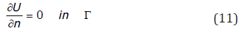
where Ω ⊂ R2 with boundary Γ , being f (x, y) a known function.
Firstly, an irregular cloud of points is generated in Ω ∪ Γ . On defining the central node with a set of nodes surrounding that node, the star then refers to a group of established nodes in relation to a central node. Each node in the domain is assigned an associated star. If U0 is the value of the function at the central node of the star and Ui are the function values at the rest of nodes, with i = 1,..., N, then, according to the Taylor series expansion in 2-D
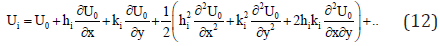
where (x0, y0) are the coordinates of the central node, (xi, yi) are the coordinates of the ith node in the star, and hi = xi –x0, ki = yi – y0. If in equation (12) are ignored the terms over the second order, an approximation of second order for the Ui function is obtained. This is indicated as ui. It is then possible to define the function B5(u) as
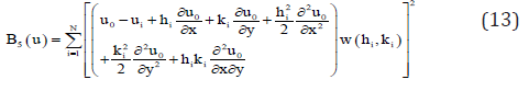
where w(hi ,ki) are positive symmetrical weighting functions , having the property as defined in Lancaster and Salkaukas [7] that are functions decreasing monotically in magnitude as the distance to the center of the weighting function increases. If the norm (13) is minimized with respect to the partial derivatives, the following linear equation system is obtained:
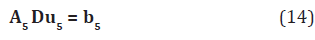
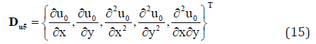
The vector Du5 is given, by:
From the previously obtained system (14) and by the fact that the matrix of coefficients A5 is symmetrical, it is possible to use the Cholesky method to solve the system. The aim is to obtain the decomposition in upper and lower triangular matrices:
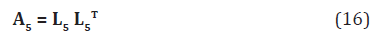
The coefficients of the matrix L5, are denoted by l(i,j) .
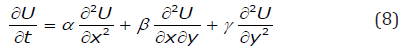
On solving the system (14), the explicit difference formulae for the partial derivatives (15) are obtained. A description of the method is given in [5]. On including the explicit expressions for the values of the partial derivatives in the right part of equations (5) or (8), the approximation equation of each point 0 taken as central node of a star is obtained:
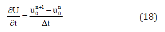
In equations (5) or (8), the first derivative of U with respect to time is approached using the explicit method by the forward difference formula
and the spatial derivatives
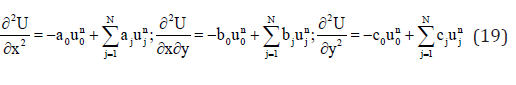
Substituting (18) and (19) into (9), we obtain
The explicit expression (22) relates the value of the function at the central node of the star, in time, with the values of the functions in the nodes of the star, for a time, multiplied by specific coefficients. This then indicates that by way of the so-called explicit method, the value of the function in a time is a weighting sum of the values of the function in the star for a time. For an explicit finite difference solution to the parabolic anisotropic PDE (9) a harmonic decomposition is made of the approximate solution at grid points at a given time level. Then, by following the von Neumann idea for stability analysis, using [12] we arrive to the following condition:
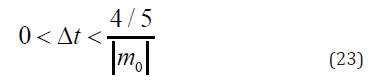
This stability condition must be accomplished for each one of the points of the domain and depends of the irregularity of the clouds of nodes used.
The operator splitting reduces the solution of the monodomain model to solving an anisotropic parabolic PDE and nonlinear systems of ODEs. To solve the nonlinear ODE systems, we apply Runge-Kutta (RK) schemes and the FitzHugh-Nagumo model. We need to solve a system of coupled ODE’s and a PDE with non-flux boundary conditions. The ODE’s solver uses local time adaptivity, allowing them to adjust the time-step. Normally, the ODE solver will take just one step for each step of the operator splitting algorithm, but in areas with rapid variations several ODE solver steps may be used in each step of the operator splitting. Let’s implement the above algorithm for cardiac tissue conduction of the two-dimensional case. The ionic current and membrane model is determined by the modified FitzHugh-Nagumo membrane kinetics (7), with a = -85, b = -68.75, c= 40, d = 0.013, e1 = 0.26/(1252), and e2 = 0.1/125. The units for U and V are mV. The spatial domain for our model is a bounded open Ω ⊂ ℝ2 with a piecewise smooth boundary ∂Ω with homogeneous Neumann boundary conditions.
This represents a two-dimensional slice of the cardiac muscle regarded as an anisotropic continuous media. We consider the case of the irregular model with 289 nodes given in Figure 1, corresponding to anisotropic material with conductivities of 0.5 and 0.1 in the fiber and cross-fiber directions respectively with a fiber angle of 45º. For the GFD explicit method, the time step used is small and the unknown variables values do not change substantially from one-time step to the next. The time-step used for the operator splitting and the GFD method has been taken according with the stability condition given previously in (23), and the Runge-Kutta methods used for the ODEs apply from 1 to 50 internal time-steps within each global step. In the monodomain equation (1) the membrane capacitance C =1. The tissue was stimulated during time steps from 10 to 20 with a current simulation Iapp =62.5 mA at different points of the tissue. Two different cases have been considered in the first one an stimulus is applied in (x0, y0) = (0.68 cm, 0.83 cm) in the center of Figure 1. The experiment in this paper was run during 60-time steps.
The output data from computer simulation can be used for further study on is potential contour lines. The iso-potentials of the numerical simulation of the first case within the domain after 20- and 60-time steps are shown in Figures 1 & 2. In the second case two stimulation points (x=0.39cm, y=0.35cm), (x=0.98cm, y=1.31cm) are considered with a current simulation Iapp =62.5 mA. In Figure 3 it is shown the location of the two stimulation points. The iso-potentials of the numerical simulation of the second case case within the domain after 20- and 60-time steps are shown in Figures 3 & 4.
Figure 1: Iso-potentials of U for the model with a fiber angle of 45º after 20-time steps.

As it is shown in the Figures 1-4 an irregular cloud of nodes is used showing the possibilities of the meshless GFDM in the modelling the monodomain equation throughout the tissue. From Figures 1-4 we clearly notice the anisotropic orientation of the fibers. The fiber angle has a great influence in the electrical propagation of the stimulus. It is easy to see there are notable changes between the two cases considered depending or the location and number of stimulation points considered.
Figure 2:Iso-potentials of U for the model with a fiber angle of 45º after 60-time steps.

Figure 3: Iso-potentials of U for the model with a fiber angle of 45º after 20-time steps.

Figure 4:Iso-potentials of U for the model with a fiber angle of 45º after 60-time steps.

In this paper we have presented a generalized finite difference method for solving monodomain equation in anisotropic medium including the condition for stability. We have suggested an explicit meshless GFD numerical method for integrating the PDE of the monodomain model used in cardiac conduction. Using implicit or semi-implicit methods this normally leads to linear systems being solved for each time step, which represents a substantial computational load. The explicit GFD approach does limit the time step size that can be used due to the stability, holding the potential of combining the geometrical efficiency of mesh-free methods with the efficiency of explicit finite difference schemes, it may therefore be a promising new approach.