info@biomedres.us
+1 (502) 904-2126
One Westbrook Corporate Center, Suite 300, Westchester, IL 60154, USA
Site Map

Received: January 31, 2019; Published: February 12, 2019
*Corresponding author: Davies Obaromi, Department of Mathematics/Statistics, Kogi State Polytechnic, Lokoja, Nigeria
DOI: 10.26717/BJSTR.2019.14.002555
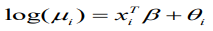
The basic model usually used in disease mapping is the Besag, York and Mollie (BYM) model, which combines two random effects, a spatially structured and a spatially unstructured random effect. Bayesian Conditional Autoregressive (CAR) model is a disease mapping method that is commonly used for smoothening the relative risk of any disease as used in the Besag, York and Mollie (BYM) model. This model (CAR), which is also usually assigned as a prior to one of the spatial random effects in the BYM model, successfully uses information from adjacent sites to improve estimates for individual sites. However, it has been pointed out that there exist some unrealistic or counterintuitive consequences on the posterior covariance matrix of the CAR prior for the spatial random effects. In the conventional BYM (Besag, York and Mollie) model, the spatially structured and the unstructured random components cannot be seen independently, and which challenges the prior definitions for the hyperparameters of the two random effects. Therefore, the main objective of this study is to utilize some spatial CAR models for flexibility as applied to tuberculosis (TB) disease mapping. The extended Bayesian spatial CAR model is proved to be a useful and a little robust tool for disease modeling and as a prior for the structured spatial random effects because of the inclusion of an extra hyperparameter. A Bayesian modeling approach by the Integrated Nested Laplace Approximation method (INLA) is used to estimate model parameters and comparison was made by the deviance information criterion (DIC).
Abbreviations: BYM: Besag, York And Mollie, CAR: Conditional Autoregressive, TB: Tuberculosis, INLA: Integrated Nested Laplace Approximation Method, DIC: Deviance Information Criterion, SAR: Simultaneously Autoregressive Model, ETR: Electronic Tuberculosis Register
Disease mapping can be described as a technique for the presentation and estimation of summary procedures of spatially observed health outcomes. The increased and improved handiness of georeferenced data and flexible computational software has increased in the application of disease mapping in the areas of epidemiology and public health [1,2]. Disease mapping can also be used to define the geographical disparity of diseases, to detect clustering of diseases and to produce diseases maps. Some authors have given a good number of statistical reviews on disease mapping [3-7]. The main and central model employed for a univariate disease mapping is the Besag, York and Mollie (BYM) model and was proposed by [8]. This model is a type of the generalized linear mixed effects model, which has two spatial random effects; one which is spatially unstructured and modeled using a normal prior and another, a spatially structured random effect which is modeled by an intrinsic conditional autoregressive (CAR) prior.
A notable challenge in spatial analyses is the problem of spatial autocorrelation. Modelling the spatial interfaces that arise in spatially referenced data is normally carried out by integrating the spatial dependence into the covariance structure either explicitly or indirectly through autoregressive models. For lattice data, the two commonly used autoregressive models are the conditional autoregressive model (CAR) and the simultaneously autoregressive model (SAR). Bayesian Conditional Autoregressive (CAR) model is a technique used in disease mapping and which is used for the smoothening of relative risk [9]. This model provides some shrink-age and spatial smoothing of the raw relative risk estimate, which gives a steadier estimate of the outline of underlying risk of disease than that given by the raw estimates. This technique effectively borrows information from neighboring areas other than from far away areas and smoothing local rates toward local neighboring values. This decreases the variance in the associated estimates and allows for the spatial effect of regional differences in State populations.
Conditional autoregressive (CAR) models are regularly used for describing the spatial variation of quantities of interest in the form of aggregates over subregions. These models have been used to analyze data in various capacities, such as in demography, economy, epidemiology and geography. The general objective of these spatial models is to show and quantify spatial relations present among the data, in specific terms, to quantify how quantities of interest differ with explanatory variables and to also to identify clusters of ‘hot spots. General versions of CAR models, a class of Gaussian Markov random fields, appear in [10-12]. CAR models have been broadly applied in spatial statistics to model observed data [13-16] as well as (unobserved) latent variables and spatially varying random effects [17,18] CAR model was first introduced by [19] and the Hierarchical disease-mapping models based on CAR was studied by [20] These CAR models yield spatial dependence in the covariance structure as a function of a neighbor matrix W, and regularly a fixed unknown spatial correlation parameter. The conditional autoregressive (CAR) and the intrinsic autoregressive models (ICAR) are extensively used as prior distributions for the structured random spatial effects in Bayesian models. However, some unrealistic or counterintuitive consequences on the prior covariance matrix or the posterior covariance matrix of the spatial random effects have been pointed out by some authors [21]. This study therefore seeks to propose, utilize and compare another latent Gaussian model, an extended CAR model, as a prior for this spatial dependency model for flexibility and better smoothing.
This is a retrospective secondary data source from Eastern Cape Province TB notification and survey data. All data used is an extract from the electronic tuberculosis register (ETR) records of TB cases from the twenty-four health sub-districts of the province including the two metropolitan municipalities. The data obtained was for the year 2014. This study was carried out in the Eastern Cape province of South Africa. The Province of the Eastern Cape is situated on the east coast of South Africa and lies between the Western Cape and KwaZulu-Natal provinces. The Northern Cape and Free State provinces, as well as Lesotho shares borders with this Province. The Eastern Cape Province boasts of amazing natural diversity, stretching from the semi-arid Great Karoo to the forests of the Wild Coast. It also extends around the Keiskamma valley, the fertile Langkloof, and the mountainous southern Drakensberg region. The main feature of the Eastern Cape is its amazing coastline adjoining the Indian Ocean. The Province covers an area of 168 966km2 and with a population of 6562 053(Statistics South Africa, Censuses 2011). The Province is situated at 32.2968°S and 26.4194°E of the country. The Eastern Cape is the second-largest province in South Africa by surface area and also the third-largest populated province with its capital in Bhisho. Port Elizabeth, East London, Grahamstown, Mthatha (previously Umtata), Graaf Reinet, Cradock and Port St Johns are the major towns and cities in the province. The province is divided into two metropolitan municipalities, and they are Buffalo City Metropolitan Municipality and Nelson Mandela Bay Metropolitan Municipality. It has six district municipalities, and which are further subdivided into 37 local municipalities.
Generally, it seems reasonable to assume that areas that are close in space show more similar disease burden than areas that are not close. To be "close" here means that we need to set up a neighbourhood structure. A well-known assumption is to regard areas i and j as neighbours if they have a common border, represented here as i˜j. This appears sensible if the regions are equally sized and organized in a regular pattern [3]. We further denote the set of neighbours of region i by δi and its size by nδi.
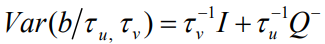
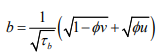
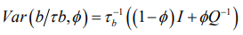
The BYM Model: The assumption of the Besag model adopts that a spatially structured component cannot take the limiting form that allows for no spatially structured variability. Hence, unstructured random error or pure overdispersion within area i, will be modelled as spatial correlation, giving confusing parameter estimates [22]. To address this issue, the Besag-York-Mollie (BYM) model [23] splits the regional spatial effect b into a sum of an unstructured and a structured spatial component, so that

Here, 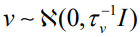 accounts for pure overdispersion, while
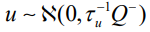 is the Besag model whereby Q− represents the generalized inverse of Q. The subsequent covariance matrix of b is
Intrinsic CAR (Besag) Model: The simplest of the CAR prior is the intrinsic model suggested by [8], which is given as
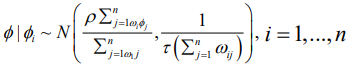 (3)
(3)where the parameter, τ, is the conditional precision. The precision is comparative to the number of neighbouring units, while the conditional expectation of ϕ_i is the mean of the random effects in the neighbouring areal units. The precision formulation here is functional, because you would expect the precision to be higher when you have more neighbouring areas and therefore more information to estimate the value of ϕi . These groups of conditional distributions agree to the multivariate normal distribution, with a zero vector mean. The improper precision matrix is given by Q=τ(diag(W1)-W), with W1, as a vector comprising the number of neighbors for each of the areal unit. One limitation of this model is the lack of a parameter to regulate the strength of the spatial autocorrelation; if you multiplied ϕ by 10, then the precision τ, would decrease, but the spatial structure does not change. This implies that the intrinsic model is only practical in circumstances where the spatial autocorrelation in the data is strong; however, it is not practical for situations where there is a weak or moderate spatial autocorrelation across the study area because the model would have a tendency to produce an overly smooth estimated risk surface in these cases
The Dean Model: [24] proposed a reparameterisation of the BYM model where
 (4)
(4)having covariance structure
 (5)
(5)Equation (5) is a reparameterisation of the original BYM model, where τ_u^ (-1) =τ_b^ (-1) ϕ and τ_v^(-1) =τ_b^(-1) (1-ϕ) [25].
A New Besag2 ICAR Model for the Structured Spatial Effects: A modification of the Dean model in (2.42) was proposed by and which addresses both the identifiability and scaling issue of the BYM model. The model uses a scaled structured component μ_(i*) where τ is the precision matrix of the Besag ICAR model. The “Besag2” is one of the models in the latent Gaussian field. The Besag2 model is an extension to the Besag (ICAR) model above in (3.14).
Let the random vector z=(x1 ,…,xn) be the “Besag” model (ICAR), then the “Besag2” is the following extensions
 (6)
(6)here a>0 is an additional hyperparameter and dim(x)=2n, and z is the same (a tiny additive noise) random vector.
This model has two hyperparameters θ= (θ1 , θ2). The precision parameter τ is represented as
 (7)
(7)And the prior is defined on θ1.
The weight parameter a is signified as
And the prior is defined on θ2 . The precision defines how equal the two copies of z is. This new prior is a member of the class of a latent Gaussian (LGMs) markov random field models and would be compared with the Besag ICAR, and the BYM models for flexibility and robustness.
Bayesian analysis rests upon computing the posterior probability distribution for model parameters. The posterior probability distribution is the conditional probability distribution of the unknown parameters, given the observed data and weighted by the prior information. Bayesian modelling depends on the ability to compute posterior distributions in order to provide estimates for all the corresponding model parameters. Majority of these posterior distributions are straightforward to calculate. Distributions with a conjugate prior typically have a posterior distribution which follows a standard distributional form.
The prior distribution is the distribution of the parameter(s) before any data is observed, that is,
The prior distribution might not be easily determined. In this case, we can use the Jeffreys prior to obtain the posterior distribution before updating them with newer observations.
The sampling distribution is the distribution of the observed data conditional on its parameters, i.e.
This is also termed the likelihood, especially when viewed as a function of the parameter(s), sometimes written,
The marginal likelihood (sometimes also termed the evidence) is the distribution of the observed data marginalized over the parameter(s),

The posterior distribution is the distribution of the parameter(s) after taking into account the observed data. This is determined by Bayes’ rule, which forms the heart of Bayesian inference

In many cases, however, the computation required is more complex and a more advanced method is essential to calculate the posterior distribution. These advanced approaches usually make use of some form of numerical simulation, generally by drawing a sample of parameter values from an approximation of the posterior distribution f(θ|Y) to allow estimation of the distributions of the model parameters (Table 1).
Table 1: Comparison of priors for the structured random effects model at 97.5% C.I without covariates.

The marginal of the posterior are not always presented in closed form as a result of the non-Gaussian response variables. For such models, Markov chain Monte Carlo methods can be applied, but they are not without some complications, both in terms of convergence and in computational time. In some practical uses, the level of these problems is such that Markov chain Monte Carlo is basically not a suitable tool for monotonous analysis.
It is shown in that by using the integrated nested Laplace approximation (INLA) method in its basic form, we can directly compute very accurate approximations to the posterior marginal. The key advantage of these approximations is simply computational, as MCMC algorithms need hours and days to run, while INLA provide more exact estimates in seconds and in minutes. Another benefit with INLA method is its generality, which makes it possible to execute Bayesian analysis in a programmed, streamlined way and to compute model comparison criteria and many predictive measures, so that models can be compared and the model under study can be tested. This method is also used where the model has a hidden Gaussian Markov Random field, with the parameters of interest being latent variables which are not observed directly but are instead inferred from other observed variables.
Considering the following hierarchical model,
 (9)
(9)Given that,φ= ( φ1,...,φn) comprise a set of random effects, which can be considered as a group of latent variables. Let be the set of hyperparameters relating to, then the marginal posterior for each variable φi is as follows:
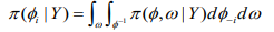 (10)
(10)where, 1 φ-1 is the vectorφ with element φi removed. This can be modified as
 (11)
(11)INLA involves the construction of a nested approximation of (5), which requires approximations of and. Here can be approximated using the following Laplace approximation
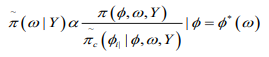 (12)
(12)where 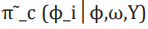 is termed the Gaussian approximation
to the full conditional distribution of and is the mode of the full conditional distribution of for a given value of . The authors in propose
using a Laplace estimate
is termed the Gaussian approximation
to the full conditional distribution of and is the mode of the full conditional distribution of for a given value of . The authors in propose
using a Laplace estimate of which takes the following
form:
of which takes the following
form:
 (13)
(13)where  is the Gaussian approximation to
and as its modal value for a given ω.
is the Gaussian approximation to
and as its modal value for a given ω.
Although in most cases similar results will be obtained by MCMC and INLA inference, it should be noted that there are fundamental differences in the way that posterior distributions are estimated. MCMC can sample directly from a joint posterior distribution, while INLA uses a closed form expression to estimate the marginal posterior distributions. For this study, we adopted the latter and the analysis was carried out in R. Models comparison were carried out using the Deviance Information Criterion (DIC), which pools together a measure of fit and a measure of model complexity based on the effective number of parameters. Smaller values of DIC show a more fitting model [26].
The comparison of numerous contending Bayesian models is usually a challenging task and needs special attention [27] Since the models used include sets of random effects, the Deviance Information Criterion (DIC) shall be used for comparison. It is defined as
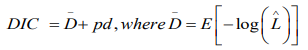
where is given as the mean posterior deviance and pd represents the actual number of parameters. When two or more models are compared, the model with the least DIC value would be adopted. Similar to the BIC, this approach penalises models which have superfluous parameters, and favours approaches which provide a sensible data fit while minimizing the amount of parameters. The best fitting model shall be the one with the smallest DIC value
Our working model is the usual BYM model which is a type of generalized linear mixed model (GLMM) with both fixed and random effects;
 (9)
(9)where b is the random effects which are further broken into spatially structured, ui, and spatially unstructured, vi, random effects. For this analysis, the standard Besag, York and Mollie convolution model is adjusted with additive spatial random effects and then used to compare the priors for the structured random effect, u_i. An offset variable, log pop, of each region i, is used as a covariate in the model.

Three (3) multilevel models with only one covariate as an offset variable are hereby developed for comparison between the spatial models BYM, the intrinsic CAR and the new “Besag2” ICAR model with additive spatial random effects and given as:


The results of a Bayesian disease-mapping analysis are presented in the form of maps displaying the spatial patterns of the three different CAR models in Figure 1. Table 1 shows the deviance information criterion for the three spatial CAR models in which the newly introduced two-parameter “Besag2” CAR model has the lesser deviance. For any model selection, deviance should be less and based on that, the Besag2 CAR model is fitted best out of the three models (Figure 2). Also, from the reparameterised “Besag2” ICAR model, which has the advantage of possessing two hyperparameters over the Besag ICAR prior with only one hyperparameter, the posterior estimates of the new prior gave significantly r educed variances for the two spatial components, and especially for the structured spatial component (σ=18.83), thereby making it to be considered as the best fit model. In terms of model choice criteria by DIC values, the three models perform at least equally well with current parameterisations, but only the Besag2 ICAR model offers parameters that are clearly interpretable and with better precision. The comparative spatial maps of the BYM and the usual ICAR models are very identical as shown in Figure 1. Spatial maps of ICAR and the new Besag2 ICAR models showed varying disease patterns when the two prior models were compared. The third model which utilized the new prior “Besag2” ICAR showed a better smooth and a more defined disease cluster and distribution. Also, the range of the posterior risks is reduced and better smoothed.
Figure 1: Posterior estimated spatial maps of the structured random prior comparisons of BYM, Besag ICAR and the new “Besag2” ICAR spatial models respectively.

Figure 2: Map of
a. Eastern Cape Province showing the 37 local municipalities and the 2 metros and
b. Extracted map from R showing the 24 health subdistricts for the TB dataset.

Disease mapping has a long history in epidemiology and one main objective is to examine the geographical distribution of disease burden. A disease mapping technique, which is usually used for smoothening of relative risk is the Bayesian Conditional Autore-gressive (CAR) model which has only one precision hyperparameter, τ. This CAR model offers some shrinkage and spatial smoothing of the raw relative risk estimate, which gives a more stable estimate of the shape of the underlying risk of disease than that given by the raw estimates [28] Without suitable weighting that is characterized with the usual ICAR prior, the hyperparameter usually have no clear meaning and may be incorrectly interpreted. This sole parameter of this ICAR rest on the basic graph structure and is confused with the mixing parameter if the structured spatial effect is not correctly scaled. Also, it is not clear on how to select a prior distribution for this precision parameter. For lack of weighting, a fixed hyperprior for the precision parameter usually give diverse amount of smoothing if the graph on which given disease counts are observed is altered [29] Also, the commonly used hyperprior distributions in the traditional ICAR prior models usually induce overfitting, and will not permit to reduce to simpler models such as a constant risk surface or uncorrelated noise over space [30] The spatially structured random effect cannot be treated individually from the unstructured spatial random effect in the classical or frequentist BYM (Besag, York and Mollie) model. This makes the prior explanations for the hyperparameters of the two spatial random effects problematic and challenging [29].
However, the major objective is not only to optimize model choice criteria such as DIC values, but to offer a sensible model design where all parameters have a clear significance and interpretation. This new model however, parameterizes the BYM model and is also an extension of the Besag ICAR model, that leads to better parameter control as the hyperparameters can be seen independently from each other. The main advantage of this novel “Besag2” ICAR model is that it permits for an intuitive parameter explanation and enables prior assignment. Also, the model is able to shrink towards a spatially unstructured risk for different disease prevalence. This shows that the Besag2 ICAR model does not overfit the parameter estimates. It is therefore acceptable, that the practical advantages in terms of interpretability and prior assignment makes the newly proposed Besag2 ICAR model in this study beneficial compared to existing models, and its usage is also recommended since its model criteria performance is better than existing approaches. The Besag2 ICAR model can be joined naturally with covariate data for use, or combined into a spatio-temporal setting [29].
Though, it will involve additional effort to allocate the variance not only within the spatial components but overall model parameters in the linear predictor. It should also be noted that the Besag2 ICAR model is not only remarkable within the context of disease mapping but also within other applications, such as genetics. Bayesian approaches provide suitable smoothing of the background rates. Mapping the raw SMRs would present a confusing and distorting picture of the risk pattern, whereas in the Bayesian models, a good posterior relative risk is obtained in all the areas [30] Generally, Conditional Autoregressive models in the Bayesian context, are useful for smoothing disease relative risk estimates based on neighborhood structures.
Davies Obaromi designed and formulated the study. Davies Obaromi drafted the manuscript, analyzed and interpreted the data.
This study was carried out under the authorization and permission of the Ethical committee of the University of Fort Hare, Alice, Eastern Cape, South Africa and approval of the Eastern Cape Department of Health, with ethical clearance reference number QIN041SOBA01 and EC_2015RP24_398 respectively.