 Review Article
ABSTRACT
This paper presents the fundamental role of the distribution of ray paths in the resolution of 2D tomographic images through the Love wave signals processing in our case study. To conduct this, we performed a 2D-linear inversion procedure on the Love wave dispersion curves and more than approximately ~25000 vertical Love wave component (Z) signals for a period range of 5 to 70 s were processed. Then, the fluctuations in resolution parameters of the 2D tomographic images include the stretching (ε) of the averaging area (L) and data density for the short-mediumlong periods were imaged and described. The results show that the resolution of tomography images is directly dependent on dense ray paths. So that, for long periods (long distances), the image resolution decreases due to the reduction of ray paths. The obtained 2D tomography images at periods of T= 5-70 s (depth-distance ~180 km) reveal that the density distribution of the signal source (transmitter-receiver of the beams or rays) and the number of ray paths in each period controls the resolution intensity and its parameters.
Keywords: Resolution; 2D Love Surface Wave Tomography; Resolution Parameters; 2D Linear Inversion
Introduction
Image resolution is the detail an image holds. The term applies to digital images, film images, and other types of images. Higher resolution means more image detail. Image resolution can be measured in various ways. Resolution quantifies how close lines can be to each other and still be visibly resolved. Resolution units can be tied to physical sizes (e.g., lines per mm, lines per inch), to the overall size of a picture, or to angular sub tense. In many biological, medical, chemical, and geophysical applications, tomography is a very useful tool for getting the one-two or three-dimensional structure of a system in large-small scales. Aside from Geophysicalmedical imaging, it has important biological applications such as getting the 3D structure of chromosomes and viruses. Medical imaging is a mathematical model of the measurement process in x-ray tomography model, that begins with a quantitative description of the interaction of x-rays with matter called Beer and the Radon transform laws. In these formulations the physical properties of an object are encoded in a function μ, called the attenuation coefficient. This function quantifies the tendency of an object to absorb or scatter x-rays. These measurements are akin to the determination of the shadow function of a convex region. In reality, the data collected are a limited part of the mathematically “necessary” data, and the measurements are subject to a variety of errors. Our study begins with a model for the interaction of Love wave rays with matter in a large-scale (a part of the Earth) and shows that these beams as they pass through different structures with increasing distance (e.g., depth, distance from source) and period are absorbed by the medium during the passage from different structures and lose their energy and it decreases the resolution of the obtained tomographic images. Literally, tomography means slice imaging. Today this term is applied to many methods used to reconstruct the internal structure of a solid object from external measurements. In 3D tomography the literal meaning persists in that we reconstruct a three-dimensional object from its two-dimensional slices (e.g., x-ray imaging, tomography from inside the earth).
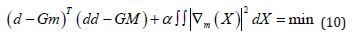
To better understand the meaning of wave absorption (damping) and to reduce the resolution of tomographic images, we first describe Beer’s law. Objects of interest in rays imaging are described by a real-valued function defined on r3, called the attenuation coefficient. The attenuation coefficient quantifies the tendency of an object to absorb or scatter x-rays of a given energy. According to Beer’s Law and ray tomography, more generally, the intensity of the beam passing through the infinitesimal area element dS, located at x, with unit normal vector n(x), is
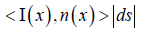
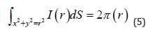
The total intensity passing through a surface S (Figures 1b & 1e) is the surface integral
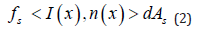
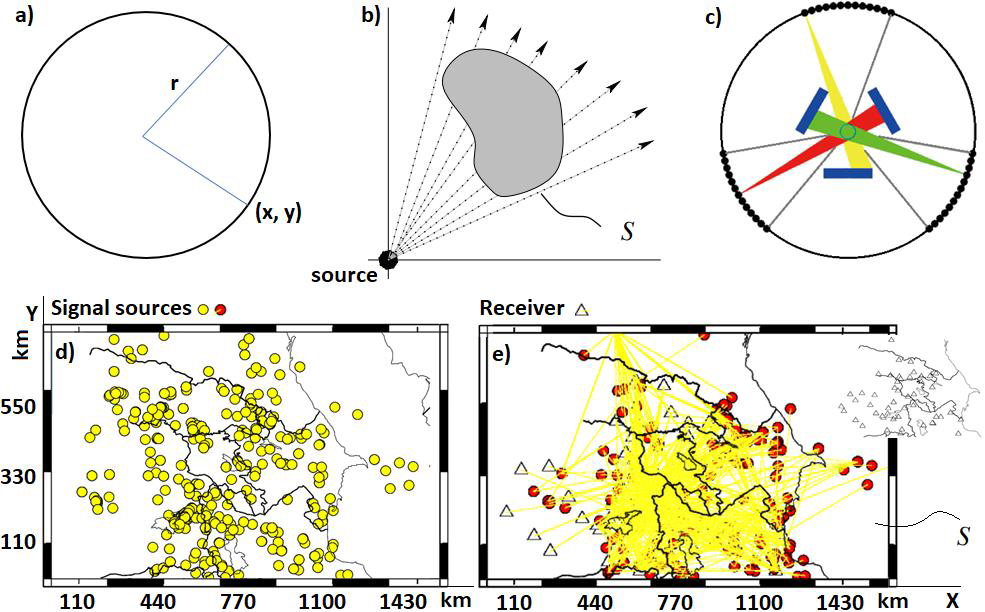
Figure 1: Analysis of an isotropic point source.
a) A point source of beams.
b) The flux through a curve not enclosing the source is zero.
c) Three examples about the shape of X-ray beam.
The yellow light path is emitted from the 13th source, the red light path is emitted from the 20th source, the green light path is emitted from the 36th source. Figures a and b are retrieved from (Thomas M. Deserno [9]) and c from (Zhicheng Zhang, et al. [10]) with slightly modifications. Figures 1 d and e show the signal sources, receivers, and ray paths used in our area S case study.
where dAs is the area element on S.
In other circumstances it is more useful to describe an x-ray as being composed of a stream of discrete particles called photons. Each photon has a well-defined energy, often quoted in units of electron-volts. The energy E is related to electromagnetic frequency by de Broglie’s Law: E = hv (3)
h is Planck’s constant.
The interaction of rays with matter is phrased in terms of the continuum model, which it rests on three basic assumptions:
1) Beams travel along straight lines that are not “bent” by the objects they pass through.
2) The waves making up the beam are all of the same frequency.
3) Each material encountered has a characteristic linear attenuation coefficient μ for beams of a given energy.
The intensity, I of the beam satisfies Beer’s law
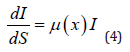
Here S is the arc-length along the straight-line trajectory of the beam (see Figures 1a-1c).
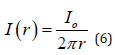
Assume that we have a point source of beams of intensity I0 in the plane. The beam source is isotropic which means the outgoing flux is the same in all directions. Because the source is isotropic, the intensity of the beam is only a function of the distance to the source. Let I (r ) denote the intensity of the flux at distance r from the source. By conservation of energy,
The intensity of the beam at distance r from the source is therefore
Finally, if a curve S does not enclose the source, then conservation of energy implies that
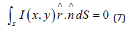
here is the outward normal vector to S. From Beer’s law and μs= 1/r attenuation coefficient see that
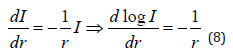
Integrating equation (8) from an r0 > 0 to r gives
This agrees with (6). That we cannot integrate down to r = 0 reflects the non-physical nature of a point source. In tomography it is often assumed that the attenuation of the beam due to beam spreading is sufficiently small, compared to the attenuation due to the object that it can be ignored. This is called a non-diverging source of beams (J. Gelijns [1]). The main purpose of this study is to prepare 2D tomographic images using Love surface wave scattering characteristics to study a large-scale area S (Caucasus territory). In this paper, we have used 2D inversion procedure to derive tomographic images of the Caucasus territory in order to better understand the internal structure activities based on increasing and decreasing wave velocity anomalies. The Love wave dispersion curves for each source-receiver path (single-receiver method) are estimated using the program do_ mft (Herrmann [2]). Then, using a method developed by (Ditmar, et al. [3]) and (Yanovskaya, et al. [4]), the 2D tomography maps are generated. To do this, we use the localregional earthquake signals recorded by the 49 broadband stations or receiver (Appendix Table 1). In our case study, this paper tries to present the fundamental role of the distribution of ray paths on the resolution of 2D tomographic images through the Love wave signals processing. To conduct this, we performed a 2D-linear inversion procedure on the Love wave dispersion curves and processed more than approximately ~25000 vertical Love wave component (Z) signals for a period range of 5 to 70 s and a depth of ~180 km. Our results show that the resolution of tomography images is directly dependent on dense ray paths. So that, for long periods (in deep surfaces or far distances), due to decreasing the number of ray paths (receivers-sources) and usually affected by scattering due to strong heterogeneity of the medium (density and elasticity) the image resolution was decreased. However, the existence of a denser sources of the beam could be helpful in determining small-scale or large-scale tomography anomalies. We should not consider long periods (T > 70 s) in the inversion procedure because of the low ray coverage.
Data and Measurements
The study area is located between 38°- 53° degrees east and
37°- 44° degrees north (Figure 2a). In this study, as mentioned, the
single-receiver method and a total of ~900 local-regional events
with magnitude  , recorded by 49 broad-bands and
short-period stations (receiver) in Seismic Network Incorporated
Research Institutions for Seismology (IRIS) stations (receiver)
, including Armenia (GNI), Georgia (GO), Turkey) (TK, TU),
Azerbaijan (AB), as well as earthquake data recorded by the Iranian
Seismological Center (IRSC), International Institute of Earthquake
Engineering and Seismology (IIEES), and temporary network of
the Institute for Advanced Studies in Basic Sciences (IASBS) as
the primary database during the period 1999 to 2018 have been
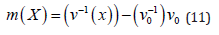
used (Appendix Table 1). (Figure 2a) shows the ray paths coverage
between station (receiver) pairs at periods of 5-70 s used for the
tomography maps computation with respective to 14 periods.
, recorded by 49 broad-bands and
short-period stations (receiver) in Seismic Network Incorporated
Research Institutions for Seismology (IRIS) stations (receiver)
, including Armenia (GNI), Georgia (GO), Turkey) (TK, TU),
Azerbaijan (AB), as well as earthquake data recorded by the Iranian
Seismological Center (IRSC), International Institute of Earthquake
Engineering and Seismology (IIEES), and temporary network of
the Institute for Advanced Studies in Basic Sciences (IASBS) as
the primary database during the period 1999 to 2018 have been
used (Appendix Table 1). (Figure 2a) shows the ray paths coverage
between station (receiver) pairs at periods of 5-70 s used for the
tomography maps computation with respective to 14 periods.
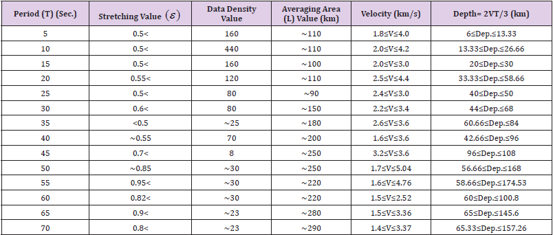
Table 1: Fluctuations in the parameters of resolution: stretching (ε ) , data density, and averaging area (L). Also the table shows the velocity (km/s) and depth (km) at periods ranging from 5 to 70 s.
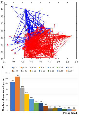
Figure 2:
a) The Ray path coverage (blue lines are the beams of the Caucasus emitted sources and red lines are for NW Iran) used to generate the 2D tomography maps. The red triangles are the receivers.
b) The number of ray paths used in the tomographic inversion respective to the period in this study.
Methods
Dispersion Estimation
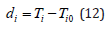
After preparing the seismic signals and preliminary correction, the group velocity dispersion curve of Love waves by applying the Herrmann’s do_mft package (Herrmann [2]) to the vertical component (Z) of motion is estimated. Modified sacmft96 work around problems with improper station (receiver) and component specifications in SAC files. Sacmft96 is called do_mft for interactive analysis of group velocities and spectral amplitudes. SAC (Seismic Analysis Code) is a general-purpose interactive program designed for the study of sequential signals, especially time series data. In fact, the frequency-time analysis of surface waves is used to estimate the dispersion curves. This method is used for estimating phase and group velocity of surface waves. It passed the preprocessed signal through a system of narrow-band filters in which the central frequency is varying and the amplitude of filter outputs is visualized in time and frequency domains. Then, on the do_mft diagram, the group velocity dispersion curve for each path is obtained. (Figures 3) shows an example of determining group velocity dispersion curve for the vertical component (Z) of the Garni (GNI) station using do_mft processing.
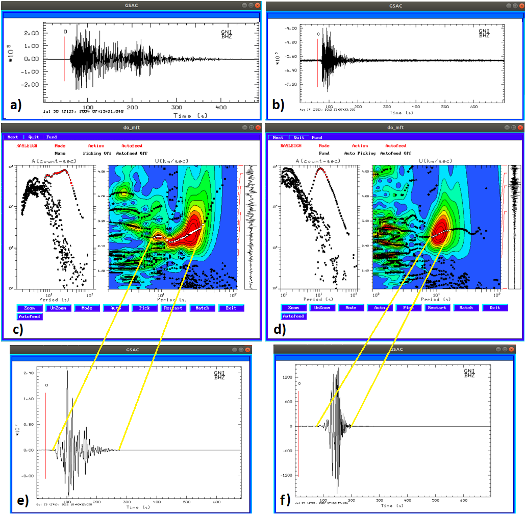
Figure 3: a and b show the raw seismogram waveforms recorded in GNI (Garni) seismic station (receiver). Figures c and d are examples of determining group velocity dispersion curve using Herrmann’s do_mft package for the vertical component (Z). The raw waveform is given in the right-hand rectangular block. Figures e and f are the cleaned waveforms related to the energetic part (red area) in figures c and d. The vertical red lines (with the number ‘0’ above them) show the chosen pickfile by SAC software (automatic default of start reading of arrival time).
To conduct this, we applied Herrmann’s do_mft package on waveforms of ~900 earthquakes recorded by the 49 stations (receiver) the Caucasus region. We then processed more than approximately ~25000 vertical component (Z) of dispersion. For this purpose, first, in Ubuntu system the data (miniSEED format) was converted to a SAC file format and then the fundamental mode of the Love waves for each vertical component (Z) using the do_mft package was determined. (Figures 3a & 3b) show the raw waveform. (Figures 3c & 3d) show the dispersion curve measurement by do_mft to separate the fundamental mode of earthquake data waveform energy, and (Figures e & f) show the cleaned waveforms related to the energetic part (red area) for an earthquake recorded in the GNI (Garni, Armenia). In the single-receiver method, since estimating the dispersion curves depends on the basic parameters of earthquakes such as magnitude, epicentral distance, depth, etc., different period ranges by applying do_mft to every epicenterstation (receiver) pair are attained; hence, for different periods we have various path numbers. Finally, a set of dispersion curves for the fundamental mode Love wave in the period range from 5 to 70 s to create 2D tomographic ray coverage maps were estimated.
Two-Dimensional Tomography
When the ground shakes at the start of an earthquake, seismic waves (signals) race outwards from it (Kinahan P, et al. [5]). In other words, the very power seismic signals are originating in Earth’s crust or upper mantle, which ricochet around the earth’s interior and travels most rapidly through cold, dense regions and more slowly through hotter rocks and materials inside the earth. Seismic tomography is like taking a Computed Tomography or CAT scan of the Earth. In a method similar to CT scans, scientists instead use seismic waves to make images of Earth’s interior. Given to the interpretation of tomography images (e.g., see https://www.iris. edu/hq/inclass/fact-sheet/seismic_tomography) from within the earth, the colors show anomalies in rigidity, which correlate with temperature anomalies. Hence, the dark blue-green-yellow shades mean colder and stiffer rock (cold spots areas) and dark red-orange shades mean warmer and weaker regions (hot spots areas). Thus, in this study, the tomography images with dark red-orange shades are low-velocity (slow-hot) and dark blue-green-yellow shades are high-velocity (fast-cold).
As mentioned, in this study, in order to construct group velocity distribution maps in period ranges from 5 to 70 s, a 2D-linear tomographic inversion technique developed by (Ditmar, et al. [3]) and (Yanovskaya, et al. [4]) was used. This methodology is a generalization of the classical 1-D method of (Backus, et al. [6]). The study region was parametrized into grids with cell size of 0.2° × 0.5° and with proper regularization parameters to provide relatively smooth maps with small data misfits. The same regularizations parameters were used for producing the maps, before and after the impoundment. The resolution of the data set is controlled by the average path length, the density of paths and the azimuthal coverage. In addition to group velocity maps, the corresponding resolution information will be provided at each period. The (Yanovskaya’s [7]) methodology is used to calculate the spatial resolution at each point and in different directions. Thus we can see, there is no need for a checkerboard test and the averaging area maps (red zones) show the most resolution.
The main advantage of this method is that in the cases of uneven distribution of surface wave paths, it works well. The dataset in this method are the travel times along different paths at each period that were calculated by the Herrmann’s do_mft package. The method estimates the lateral variation of group velocity x v at each period. The lateral group velocity distribution could be estimated by minimizing the following function:
Were
Were
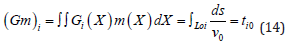
In the relations (10–14), X = (θ, φ) is the position vector, V0 is the velocity corresponding to a starting model, ti is the observed travel time along the path, io t s the travel time calculated for the starting model, α is a regularization parameter, io t is the length of the th t path and s is the segment along which the inversion is performed. The regularization parameter (α) that depends on the accuracy of the data, is the trade-off between the fit to the data and the smoothness of resulting velocity distribution. Decrease in α gives a sharper solution region with an increase in solution error, whereas increase in α leads to smoothing of the solution region with decrease in solution error (Yanovskaya, et al. [8]). The parameter α controls the trade-off between the fit to the data and the smoothness of the resulting group velocity maps. Therefore, to improve the resolution and for having a real model, we tested various values of the regularization parameter. We chose α = 0.2 that gives relatively smooth maps with small solution errors which was conducted by testing different α values and observing the number of rays passing through each cell size of 0.2° × 0.5° by running the specialized computer codes in MATLAB software which used in this study. Finally, by using the GSAC, GMT software, and computer specialized codes in the Ubuntu operating system and MATLAB software, the 2D tomography ray coverage, stretching, data density, and averaging area maps were plotted and estimated in period ranges from 5 to 70 s.
Ray Paths Distribution and Resolution Parameters
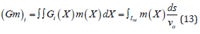
The resolution of the data set is controlled by the average path length, the density of paths and the azimuthal coverage. The resolution of group velocity maps depends more on the density of the paths and their balance distribution (crossing paths). In tomographic studies related to signal data, these two parameters depend on the geometry of the seismic array (receivers) and on the distribution of the signal sources that can limit the number of available paths for some directions which is almost beyond our control (see Figure 1). (Figure 4) shows the ray path distribution at periods 5-70 s and (Figure 2a) shows the total number of ray paths for the selected periods which were used in this study to create the tomographic images. For periods between 5-30 s, the ray path is larger than 4500 (Figure 2b). The dense ray path distribution (Figure 5- averaging area) controls the reliability and the high resolution of tomography results (red shads). Hence, for different periods, there are different number of paths. The (Table 1) and (Figure 5) show the changes in resolution parameters include the stretching ex or ɛ the averaging area (L) and data density for the short-medium-long periods.
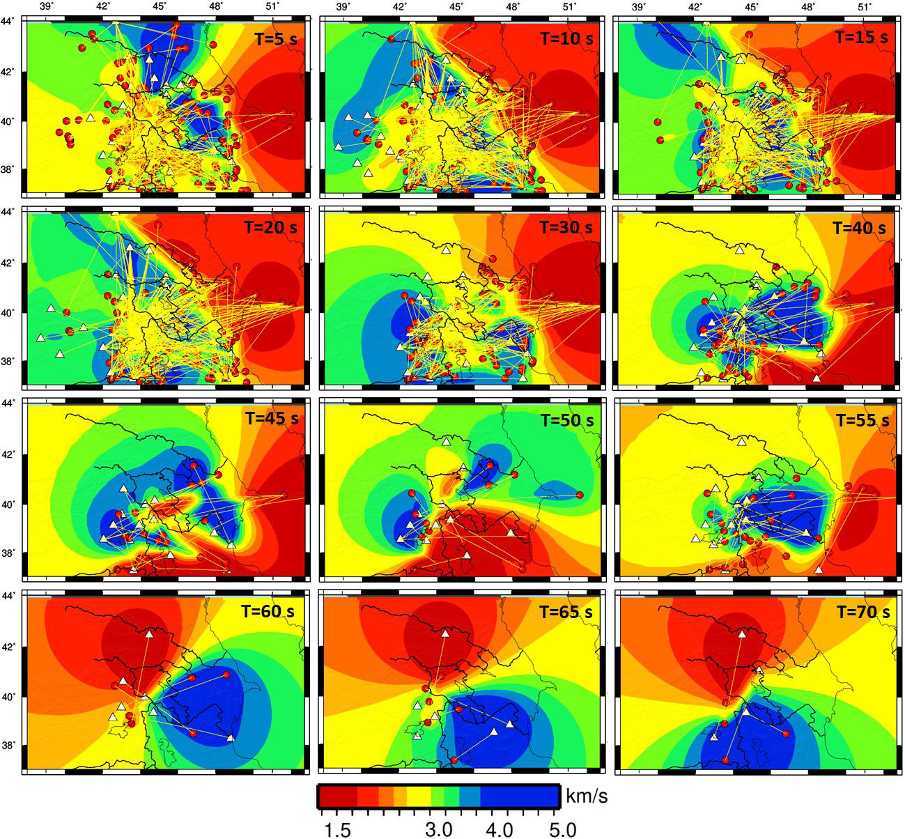
Figure 4: Ray paths for Love wave signals) rays were obtained from ~25000 vertical components (yellow cross) and 900 signal sources or seismic events (yellow-red circles) recorded by 49 receivers (white triangle). The resolution of short-medium periods is much better than that of longer period maps, in which the dense ray path distribution controls the high resolution of tomography maps. The maps at period 60, 65, and 70 s (butterfly-shaped areas) because of the poor coverage of ray paths has resulted in smearing the feature toward the Southeast-Northwest (at periods 60-65 s), and South-North (at period 70 s).
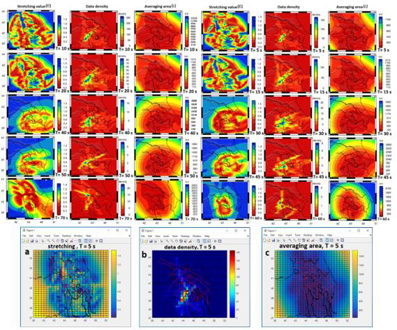
Figure 5: Resolution of data as mean size of the averaging area (L), stretching (ɛ) of the averaging area, and data density at different short (5, 10s)- medium (40, 45s)- long (60, 70s) periods. In the averaging area maps, the red zones have the most resolution. Figures a, b and c show the cell size of 0.2° × 0.5° (20 × 50 km2) for the resolution parameters at period 5 s (generated by MATLAB software).
According to (Yanovskaya [7]) and (Yanovskaya, et al. [8]), the stretching of the averaging area and the mean size parameters are used to estimate the lateral resolution. For 2D tomography problems, a function S (x, y) for different orientations of the coordinate system is used in order to determine the sizes of the averaging area along different directions. The averaging area which gives us an idea of the obtained resolution can be approximated by an ellipse centered at a point, with axes equal to the largest Smax (x, y) and to the smallest Smin (x, y) values of S (x, y). The smallest Smin (x, y) and largest Smax (x, y) axes of the ellipse are calculated, and the resolution in each point is given the mean size of the averaging area:
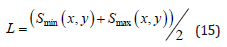
As the resolution is closely correlated to the density of the crossing ray paths in each cell, it is clear that small values of the mean size of the averaging area (corresponding to high resolution) should appear in the areas that are crossed by a large number of raypaths and vice versa. The second parameter is the stretching of the averaging area, which provides information on the azimuthal distribution of the ray paths and is given by the ratio:
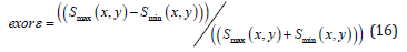
Where max S and min S are the large and small elliptical focal lengths. (Figures 5a - 5c) shows the cell size of the 0.2° × 0.5° (20 × 50 km2) for the stretching, data density, and averaging area parameters at period 5 s (generated by MATLAB software). According to study (Yanovskaya [7]), large values of the stretching parameter (usually > 1) imply that the paths have a preferred orientation and along this preferential direction is likely to be quite small. On the contrary, small values of the stretching parameter imply that the paths are more or less uniformly distributed along all directions; hence the resolution at each point can be represented by the mean size of the averaging area. In our study, = 182.857 and exorε = 0.6985 ≅ 0.7were obtained. Distribution of stations (receiver) and earthquakes controls the amount of stretching parameter and data density. The mean size of the averaging area of our tomographic results is of the order of 20 km in most of the study region. The values of the stretching of the averaging area are between 0.5 and 0.95 in most of the study area at the fourteen periods. This indicates that the azimuthal distribution of the paths is sufficiently uniform and that the resolution is almost the same along any direction. For periods between 5-70 s, the ray path averaging area is larger than ~150, with its maximum equal to ~2400 (Figure 5).
Discussion
Tomography (e.g., medical, geophysics, industrial CT systems) is a technique which is used to generate 3D images of the inside of the various bodies (e.g., human body, Earth) and thus represents one of the most powerful tools to explore objects interior. Seismic tomography has its roots in the computed tomography (CT) scanning, a technique used in medicine to look inside the human body. Although the underlying theory is quite similar, in the medical imaging case, the source and receiver distribution is controlled by the operator, unlike the seismology where we can only control the locations of the receivers. It is possible to use much more extensive observational material by incorporating data over mixed paths, i.e., the ones traversing regions of different structures (various material) [9]. If the ratio between the segments of a path corresponding to different regions varies with the path, then the tomography anomalies in each region can be estimated from the wave absorption (rays) for such paths. This possibility is based on the homogeneous medium within each region (the boundaries between them are known), which in this case the effects of refraction and phase distortion at boundaries can be neglected. Also, surface waves are dispersive- which means that different periods travel at different velocities. Hence, surface waves with different periods are sensitive to seismic wave velocities at different depths, and waves with the longer period are sensitive to greater depths [10]. These results indicate velocity structure variations for different periods, so that the lower periods for the thin and lower depths (distance) and higher periods for high depth (distance) areas is sampled. Distribution of receivers and signal sources controls the amount of stretching parameter and data density.
The mean size of the averaging area of our tomographic results is of the order of 20 km in most of the study region. The values of the stretching of the averaging area are between 0.5 and 0.95 in most of the study area at the fourteen periods. This indicates that the azimuthal distribution of the paths is sufficiently uniform and that the resolution is almost the same along any direction. For periods between 5-70 s, the ray path averaging area is larger than ~150, with its maximum equal to ~2400. In our study, L = 182.857 and ex or ɛ=0.6985≅0.7 were obtained. At short-periods (5 ≤ T ≤ 40 s; short distances), the obtained 2D ray path tomography maps, due to dense ray paths mainly reveal the structures and layers with shallow-thin textures (soft and hard). In the long-medium periods (45 ≤ T ≤ 70 s; far distances) of our case study, the 2D ray path tomographic maps, due to sparse and poor ray paths the images resolution is low and it controlled by structures and layers with deep-thick textures. On the other hands, in our tomography ray path maps, the red-orange shades show the warmer and weaker regions (hot spot areas) and dark blue-green-yellow shades mean colder and stiffer rock (cold spot areas).
Conclusion
The resolution length (averaging area- L) results are on the order of 50-200 km for the most parts of the study area (Figure 5), but for the marginal areas with low ray coverage, these values are even more. The stretching parameter values are spatial distribution (azimuthal coverage) of the paths, and large values of this parameter show a preferred orientation of the paths. The distribution of the stations (receiver) and earthquakes controls the stretching parameter. The smaller value of that (usually <1) indicates a uniform distribution of rays. Its value in our results is about 0.7, which shows a uniform distribution and an identical resolution along each path for most parts of the study area (Figure 5 and Table 1). Also, from the ray path tomography maps obtained in our case study (Figure 4), the resolution of short-medium periods is much better than that of longer period maps, in which the dense ray path distribution controls the high resolution of tomography maps. At short periods (e.g., T < 25 s) surface waves sample the shallower structure, while at long periods (e.g., T > 50 s) surface waves are mainly sensitive to the structure at large depth.
References
- J Gelijns (2010) Computed Tomography, IAEA publication (ISBN 978-92-0-131010-1).
- RB Herrmann (2013) Computer Programs in Seismology: An Evolving Tool for Instruction and Research. Seis Res Lettr 84(6): 1081-1088.
- Ditmar PG, Yanovskaya TB (1987) Generalization of Backus-Gilbert method for estimation of lateral variations of surface wave velocities: Phys. Solid Earth, Izvestia Acad Sci USSR 23(6): 470-477.
- Yanovskaya TB, Ditmar PG (1990) Smoothness criteria in surface wave tomography. Geophys J Int 102(1): 63-72.
- Kinahan P, Townsend D, T Beyer, D Sashin (1998) Attenuation correction for a combined 3D PET/CT scanner. Med Phys 25(10): 2046-2053.
- Backus G, Gilbert F (1968) The resolving power of gross Earth data. Geophys J R astr Soc 16(2): 169-205.
- Yanovskaya TB (1997) Resolution estimation in the problems of seismic ray tomography, Izv. Phys. Solid Earth33(9): 762-765.
- Yanovskaya TB, Kazima E, Antonova L (1998) Structure of the crust in the Black Sea and adjoining region. J Seismol 2(4): 303-316.
- Thomas MD (2011) Biomedical image processing,
- Zhicheng Zhang, Shaode Y, Xiaokun L, Yanchun Z, Yaoqin X, et al. (2016) A novel design of ultrafast micro-CT system based on carbon nanotube: A feasibility study in phantom. Physica Media 32(10): 1302-1307.
