Morphing from the TV-Norm to the l₀-Norm Volume 55- Issue 1

Gengsheng L Zeng^1* and Ya Li²

• ¹Department of Computer Science, Department of Radiology and Imaging Sciences, Utah Valley University, USA
• ²Department of Mathematics, Utah Valley University, USA

Received: February 07, 2024; Published: February 21, 2024

*Corresponding author: Gengsheng L Zeng, Department of Computer Science, Department of Radiology and Imaging Sciences, Utah Valley University, Orem, Lake City, UT 84058 USA

DOI: 10.26717/BJSTR.2024.55.008665

Abstract PDF

ABSTRACT

For piecewise constant objects, the images can be reconstructed with under-sampled measurements. The gradient image of a piecewise image is sparse. If a sparse solution is a desired solution, an l₀-norm minimization method is effective to solve an under-determined system. However, the l₀-norm is not differentiable, and it is not straightforward to minimize an l₀-norm. This paper suggests a function that is like the l₀-norm function, and we refer to this function as meta l₀-norm. The subdifferential of the meta l0-norm has a simple explicit expression. Thus, it is straightforward to derive a gradient descent algorithm to enforce the sparseness in the solution. In fact, the proposed meta norm is transition that varies between the TV-norm and the l₀-norm. As an application, this paper uses the proposed meta l₀-norm for few-view tomography. Computer simulation results indicate that the proposed meta l₀-norm effectively guides the image reconstruction algorithm to a piecewise constant solution. It is not clear whether the TV-norm or the l₀-norm is more effective in producing a sparse solution. Index Terms—Inverse problem, optimization, total-variation minimization, l₀-norm minimization, few-view tomography, iterative algorithm, image reconstruction

Abbreviations: SSIM: Studies with Structure Similarity; PSNR: Peak Signal-to-Noise Ratio; SNR: Signal-to-Noise Ratio; MLEM: Maximum-Likelihood Expectation-Maximization; POCS: Projections onto Convex Sets

Introduction

COMPRESSED sensing is a technology to use under-sampled measurements for solving an inverse problem [1-4]. When the measurements are insufficient, the imaging system is underdetermined, and the object to be imaged is not well defined. Extra information is required for a useful reconstructed image. For certain objects, extra information is available. The sparseness of an object is an important piece of information. An image array is said to be sparse if most of the array elements are zero. For example, the edge image of piecewise constant images is sparse. Let us consider the following situation. The desired solution, X, of an inverse problem is sparse after a certain sparsifying transformation ψ, that is, ψ(X) is sparse. The sparseness is measured by the l₀ norm, ‖∙‖₀ . If X is a vector,

the total number of nonzero elements in 𝑋. (1)

If X is a scalar, ‖𝑋‖₀ is a binary number as

An under-determined inverse problem has infinitely many solutions. A compressed sensing solution is a solution with a minimum

value.

Mathematically speaking, the l0 norm is not really a norm nor even a pseudo-norm, because, in general,

In this paper, we use the term ‘norm’ loosely. The difficulty of using the l₀-norm is that the l₀-norm is nondifferentiable. Many researchers have attempted to tackle the l₀-norm minimization problem. The work in [5] converted the l₀-norm minimization problem into an unconstrained augment Lagrange problem. The work in [6] solved the l₀-norm minimization problem by introducing auxiliary variables. The l₀-norm minimization solution used in [7] involved a hard thresholding, linearization, and proximal points techniques. The l₀-norm minimization is usually achieved by solving some sub problems [8]. Due to the difficulty in minimizing the l₀-norm, the total variation (TV) norm minimization, which is the l1-norm of the gradient, has been given more attention [9-11]. This is because the implementation of the l₁-norm optimization is much easier that the l₀-norm optimization. The main purpose of this current paper is to present a simple way to implement the l₀-norm optimization.

Methods

The l₀-Norm and Proposed Meta l₀-Norm

In our two-dimensional (2D) image reconstruction applications, we choose the finite differences in the row and column directions as the sparsifying transformation ψ . Let the 2D image be X and its pixels be denoted as 𝑥_𝑖,𝑗, where i is the row index and j is the column index. At each pixel, ψ(𝑥_𝑖,𝑗) is a finite difference gradient, which is a 2D vector

The optimization metric (i.e., the objective function) can be set up as the sum of the l₀-norm of all pixels in the image as

One difficulty of minimizing (5) is that the l0-norm is not differentiable and is not easy to optimize. One common method to mitigate the difficulty is to use the l1-norm approximation [9-13]. The famous total variation (TV) method is to use the l1-norm of the finite difference gradient to replace the l0-norm of the finite difference gradient. For a 2D image X, the isotropic TV norm is defined as

and the anisotropic TV norm is defined as

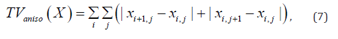
This paper proposes an alternative ‘norm’ to replace the l₀-norm. We refer to the proposed ‘norm’ as the meta l₀-norm, which is defined for a scalar X as

where 0 < a < ∞ is user-defined parameter. When 𝑋 = 0, ‖𝑋‖_{𝑚𝑒𝑡𝑎0} = ‖𝑋‖₀ = 0. When 𝑋 ≠ 0, ‖𝑋‖_{𝑚𝑒𝑡𝑎0} ≈ ‖𝑋‖₀ = 1 if 𝑎 is chosen large enough. Figure 1 illustrates the approximation of ‖𝑋‖₀ by proposed ‖𝑋‖_{𝑚𝑒𝑡𝑎0} .

For a 2D vector

we define the anisotropic meta l₀-norm as

and define the isotropic meta l₀-norm as

For a 2D image X, we replace (5) by the anisotropic metric

or the isotropic metric

The subdifferential exists for the proposed metric (11) as

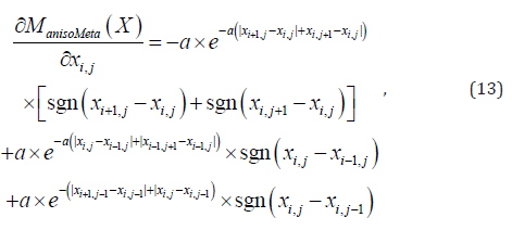
where the sign function in (13) is defined as

The subdifferential given in (13) readily leads to a gradient descent algorithm to minimize the metric given in (11). The subdifferential for (12) can be similarly obtained.

Application: Few-View Tomography

Here we consider a 2D parallel-beam imaging system, where the image array was 256 × 256, the detector contained 256 bins, and the number of views over 180° was 30. The noiseless projection line integrals were generated analytically (without using pixels). A method based on ‘projections onto convex sets’ (POCS) was selected to reconstruct the image. This method alternated between the maximum-likelihood expectation-maximization (MLEM) image reconstruction algorithm and a gradient descent algorithm that minimized the metric 𝑀_{𝑎𝑛𝑖𝑠𝑜𝑀𝑒𝑡𝑎}(𝑋) or 𝑀_{𝑖𝑠𝑜𝑀𝑒𝑡𝑎}(𝑋). There were 200 iterations used in the POCS algorithm. At each POCS iteration, there were 5000 iterations for the gradient descent algorithm. A flow chart of the algorithm is illustrated in Figure 2. In the computer simulations, the Shepp-Logan phantom was used [14]. In addition to the noiseless data set, a noisy data set was also generated with the zero-mean Gaussian noise added.

In Figure 2, the image reconstruction algorithm ① is the MLEM algorithm:

where 𝑝_𝑚 is the mth projection, 𝑎_{𝑖,𝑗,𝑚} is the projection contribution from the pixel (i,j) to the projection bin m, and k is the iteration index. In fact, the user can choose any iterative image reconstruction algorithm for algorithm ①. The gradient descent algorithm ② in Figure 2 is given as

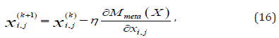
where 𝜂 = 2 × 10⁻⁷ in our computer simulations, and

is defined by (13) or

. The number of iterations shown in Figure 2 is served as an example only. A TV constrained image reconstruction algorithm was also implemented for the comparison purposes. The TV implementation was in the same format as depicted in Figure 2, except that the gradient

was calculated with the TV norm (6) or (7).

Results

The reconstructions via the MLEM, anisotropic/isotropic TV, and the proposed anisotropic/isotropic meta l₀ method are shown in Figures 3 & 4, respectively, for the noiseless and noisy data. Tables 1-4 show the quantitative comparison studies with structure similarity (SSIM), peak signal-to-noise ratio (PSNR), and signal-to-noise ratio (SNR). When the parameter ‘a’ is small, the proposed meta l0-norms behave like TV norms. On the other hand, when the parameter ‘a’ is large, the meta l₀-norms behave like the l₀-norms. Thus, the proposed meta l₀-norm are snapshots of the morphing from the TV norm to the l₀-norm for different ‘a’ value. When a = 10000, the numerical values of the exponential function become underflow. The constraints are not effective and are ignored. It is observed that the l₀-norm give better SSIM results. However, the TV norms give better PSNR and SNR results. Therefore, we cannot conclude whether the TV norms or the l₀-norms are the better choices for sparse solutions.

Discussion and Conclusions

Simple meta l₀-norms are suggested in this paper to replace the l₀-norm in searching a sparse solution for an inverse problem with under-sampled data. Thess meta norms have a user defined parameter ‘a’. The meta l₀-norms behave like the l₀-norm when ‘a’ is large. The most significant advantage of the meta l₀-norms is that it is subdifferentiable. Therefore, it is straightforward to derive a gradient descent algorithm to minimize the meta l₀-norms. Computer simulations in this paper show that the meta l₀-norms are effective in producing a piecewise solution. The meta norms are snapshots between the TV norms and the l₀-norms. The choice of a better norm is task dependent. The l₀-norms are not always preferred. We must point out that the l₀-norm minimization problem is far from being solved. The l₀-norm minimization problem is NP-hard. The gradient descent algorithm to minimize the meta l₀-norms is merely a greedy approach. The l₀-norm minimization problem has multiple minima. Any gradient based methods can only find a local minimum.

References

1. DL Donoho (2006) For most large underdetermined systems of linear equations the minimal 1-norm solution is also the sparsest solution. Communications on Pure and Applied Mathematics 59(6): 797-829.
2. DL Donoho (2006) Compressed sensing, IEEE Transactions on Information Theory 52(4): 1289-1306.
3. EJ Candès, JK Romberg, T Tao (2016) Robust uncertainty principles: Exact signal reconstruction from highly incomplete Fourier information. IEEE Trans Inf Theory 52(8): 489-509.
4. LI Rudin, S Osher, E Fatemi (1992) Nonlinear total variation-based noise removal algorithms. Physica D: Nonlinear Phenomena 60(1-4): 259-268.
5. H Chen, J Tao, Y Sun, Z Ye, B Qiu, et al. (2015) Magnetic resonance image reconstruction via L0-norm minimization. 2015 IET International Conference on Biomedical Image and Signal Processing (ICBISP 2015), Beijing p. 1-6.
6. Li Xu, Cewu Lu, Yi Xu, Jiaya Jia (2011) Image smoothing via L0 gradient minimization. ACM Transactions on Graphics 30(6): 174.
7. Y Sun, J Tao (2014) Few views image reconstruction using alternating direction method via L0-minimization International Journal of Imaging Systems and Technology 24: 214-223.
8. Wei Yu, Li Zeng (2015) ℓ₀ gradient minimization-based image reconstruction for limited-angle computed tomography. PLOS ONE 10(7): e0130793.
9. Xuan Fei, Zhihui Wei, Liang Xiao (2013) Iterative directional total variation refinement for compressive sensing image reconstruction. IEEE Signal Processing Letters 20(11): 1070-1073.
10. EY Sidky, X Pan (2008) Image reconstruction in circular cone-beam computed tomography by constrained, total-variation minimization. Physics in Medicine & Biology 53: 4777-4807.
11. VP Panin, GL Zeng, GT Gullberg (1999) Total variation regulated EM algorithm. IEEE Trans Nucl Sci 46(6): 2202-2210.
12. GL Zeng, Y Li, A Zamyatin (2013) Iterative total-variation reconstruction versus weighted filtered-backprojection reconstruction with edge-preserving filtering. Phys Med Biol 58: 3413-3431.
13. GL Zeng (2022) A projection-domain iterative algorithm for metal artifact reduction by minimizing the total-variation norm and the negative-pixel energy. Visual Computing for Industry Biomedicine and Art 5:1.
14. LA Shepp, BF Logan (1974) The Fourier reconstruction of a head section. IEEE Transactions on Nuclear Science NS-21(3): 21-43.